


Dynamic Chunking for End-to-End Hierarchical Sequence Modeling | Summary
10 Jul 2025 | Paper Review Sequence Modeling Tokenization State Space ModelsContents
Version note. This manual retrospective review covers a paper selected for 2025-W28 using arXiv v2, dated 15 July 2025. That revision appeared after the selected week; the discussion below describes v2.
This article explains Dynamic Chunking for End-to-End Hierarchical Sequence Modeling by Sukjun Hwang, Brandon Wang, and Albert Gu.
- 2025-07-10 (original arXiv release)
- Carnegie Mellon University, Cartesia AI
- Paper, arXiv v2
Image attribution. Source: Sukjun Hwang, Brandon Wang and Albert Gu, Dynamic Chunking for End-to-End Hierarchical Sequence Modeling, arXiv:2507.07955v2. The arXiv record lists the paper under CC BY 4.0. The images are cropped from the source PDF: Figures 1 and 2 (pp. 3 and 7), and Table 2 (p. 13).
Summary
- H-Net learns where to compress a byte sequence instead of relying on a fixed tokenizer. An encoder produces detailed representations, a router selects context-dependent chunk boundaries, and a main network processes the shorter sequence before a decoder restores the original resolution.
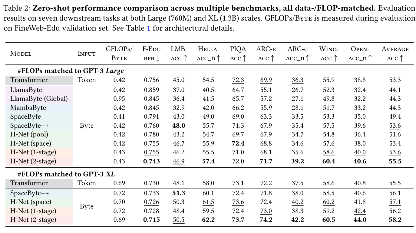
- In Table 2, with training data and FLOPs matched, the two-stage H-Net has FineWeb-Edu validation bits per byte (BPB) of 0.743 versus 0.756 for a BPE Transformer at the Large setting, and 0.715 versus 0.730 at XL. Lower BPB is better. The seven-task average is 55.5 versus 53.3 and 58.2 versus 55.5, respectively.
- The experiments also cover text perturbations, Chinese, code, and DNA. The authors report training and memory costs. The largest two-stage H-Net in the main experiments has 1.6B parameters and is FLOP-matched to a 1.3B Transformer; those experiments do not establish scaling from scratch at larger model sizes.
1 Introduction
Byte-pair encoding (BPE) compresses text into a shorter sequence, making language models cheaper to train. Its vocabulary and segmentation are fixed before model training, however, and the same choices need not suit every language or modality. Direct byte-level models avoid that preprocessing but must process longer sequences. Previous hierarchical approaches shorten the sequence with fixed pooling or hand-designed boundary rules; the paper asks whether the model can learn the boundaries jointly with the task.
H-Net combines hierarchical processing with dynamic chunking. Its main network works on a compressed sequence, while smaller outer networks retain detail at the original resolution. The main experiments study both one and two compression stages and learn boundaries without supervised segmentation labels.
2 H-Net Architecture
2.1 Architectural overview
Each stage has an encoder, a chunking layer, a dechunking layer, and a decoder. The encoder processes the incoming sequence; chunking selects a shorter sequence for the next stage or main network. Dechunking expands the main-network output, adds a projected encoder residual, and passes the result to the decoder. Repeating this structure creates multiple levels of compression. Figure 1 on page 3 illustrates a two-stage model.
The left panel traces compression and reconstruction through two stages. The right panel separates boundary routing and downsampling from smoothing and upsampling.
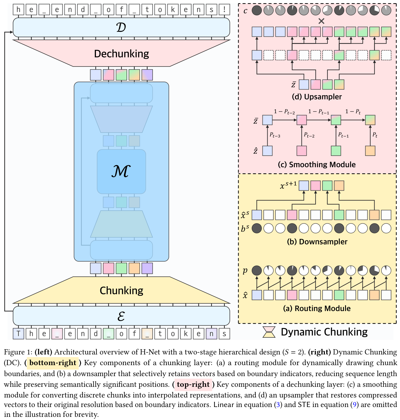
The paper uses Mamba-2 state-space layers in the encoders and decoders, which operate on longer sequences, and a Transformer as the default main network. Most parameters are allocated to the compressed main stage. The architecture is modular, so the main network can also use another sequence model.
2.2 Dynamic chunking
The router applies separate learned projections to adjacent encoder representations and scores their cosine similarity. Lower similarity between the projected representations yields a higher boundary score, allowing boundaries to depend on the current data and context. The downsampler selects the representations at those boundaries. A separate auxiliary loss encourages a target compression ratio; it does not provide ground-truth word boundaries.
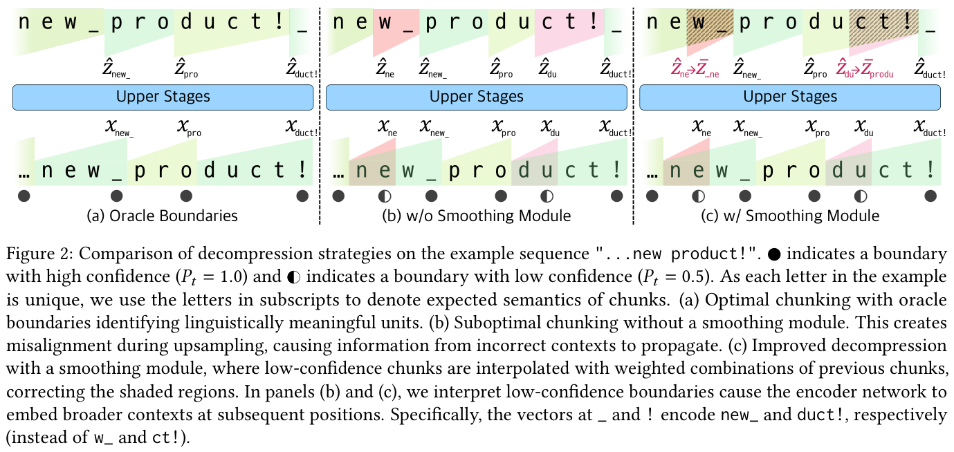
Dechunking must propagate information back to every original position. The smoothing module interpolates representations from earlier chunks according to boundary confidence, so an uncertain boundary has a softer effect than a confident one. Figure 2 on page 7 illustrates the alignment problem and the effect of smoothing. A straight-through estimator preserves a discrete forward choice while allowing a gradient signal to reach the router.
The example compares ideal boundaries with an uncertain boundary before and after smoothing. Filled circles indicate high boundary confidence and half-filled circles indicate low confidence.
2.3 Stable hierarchical training
The authors adjust projection and normalization placement to balance signals between the networks. They also adapt optimization settings to layer width and the effective batch size at each compressed stage. These choices address interactions between the outer networks and the more heavily parameterized main network; they are part of the reported training setup, not a separate evaluation dataset.
2.4 Autoregressive training and inference
The model predicts sequences autoregressively. At inference, routing determines whether a new position needs computation in the compressed main stage, while the outer networks continue at the original resolution. The chunking and dechunking operations are designed to preserve causality, so a prediction does not use future input.
3 Experiments
3.1 Language modeling and robustness
The English experiments compare models at matched training data and computational budgets, with FLOPs matched to GPT-3 Large (760M parameters) and GPT-3 XL (1.3B parameters). Training uses a 100B-token FineWeb-Edu subset, a batch size of 256, and sequences of 8,192 UTF-8 bytes for byte models versus 1,792 GPT-2 tokens for the baseline, approximately the same number of bytes. Table 2 reports both FineWeb-Edu validation BPB and zero-shot results on seven downstream tasks. At the Large setting, the two-stage H-Net scores 0.743 BPB and a 55.5 task average, compared with 0.756 and 53.3 for the tokenized Transformer. At XL, the corresponding values are 0.715 and 58.2 versus 0.730 and 55.5.
The authors caution that the BPE baseline’s BPB calculation uses the probability of the greedy tokenization as an approximation to the probability of the string. Other tokenizations can represent the same string, so this estimate overstates BPE BPB; exact computation is intractable in their setting. The downstream task results are separate measurements.
The two model-size sections report validation BPB and seven downstream task scores under matched training budgets. Lower BPB and higher task accuracy are better.
On HellaSwag with five kinds of text perturbation, the authors evaluate checkpoints trained on clean data without noise augmentation. Table 3 reports a Large H-Net average of 38.0 and robustness score of 39.0, compared with 30.9 and 20.2 for the Transformer. At XL, the respective values are 40.9 and 42.8 versus 32.3 and 22.2. The robustness score is the paper’s metric and should not be confused with the average accuracy.
Visualizations of learned boundaries show frequent boundaries around spaces as well as content-dependent grouping across words. These examples illustrate learned behavior; they do not prove that every resulting chunk corresponds to a linguistic unit.
3.2 Other languages and modalities
Table 4 reports Chinese validation BPB of 0.7032 for H-Net versus 0.7404 for the BPE Transformer, and XW-zh scores of 0.663 versus 0.599. For code, the reported BPB values are 0.3161 and 0.3376. These comparisons use the paper’s particular datasets and matched-budget setup.
For the HG38 DNA experiment, Table 5 reports H-Net perplexities of 2.705 and 2.697, compared with 2.769 for the Transformer and 2.757 for Mamba-2. Figure 6’s caption estimates that H-Net needs approximately 3.6 times less data for comparable performance in the stable training region. The adjacent discussion instead says “3.6× the amount of data” without “less”; the two wordings do not agree. The introduction and Appendix E.3 describe a 3.6-fold improvement in data efficiency. The H-Net variants have 64M and 66M parameters, compared with 29M for the Transformer and 33M for Mamba-2; this is not an equal-parameter comparison. It is specific to this DNA setup, not a general guarantee for all biological sequences.
3.3 Ablations
The ablations examine encoder and decoder choices, chunking strategies, smoothing, and hierarchy. The reported comparisons support the combination of state-space outer networks and learned chunking in the tested settings. Fixed pooling and space-based boundaries provide useful reference points: H-Net’s advantage depends on both architecture and the learned compression mechanism, rather than on removing a tokenizer alone.
4 Discussion
Dynamic sequence lengths complicate batching and memory allocation. The authors report that their implementation can train up to roughly twice as slowly as an isotropic model and that long batches can cause out-of-memory failures. They did not test a three-stage hierarchy or train larger main-experiment models from scratch. Appendix F separately explores distillation using a frozen Llama 3.2 3B main network and boundary supervision; it is a different setting from the main experiments. The data-scaling comparison uses a stable region as a proxy rather than a full scaling-law study.
5 Conclusion
H-Net offers a way to learn segmentation jointly with a sequence model while concentrating computation on compressed representations. Its matched-budget experiments show improvements over the stated tokenized baseline in several settings, with practical training costs and scale limits that remain part of the result.