LLM in a flash: Efficient Large Language Model Inference with Limited Memory | Summary

This article explains the key points of LLM in a flash: Efficient Large Language Model Inference with Limited Memory.

• 2023-12-12 (arXiv)
• Alizadeh, Keivan, Mirzadeh, Iman, Belenko, Dmitry, Khatamifard, Karen, Cho, Minsik, Del Mundo, Carlo C, Rastegari, Mohammad, Farajtabar, Mehrdad.
• Apple
• Paper

Read this article in Korean

Summary

• Running a large language model (LLM) becomes difficult when its weights exceed available dynamic random-access memory (DRAM), the device’s working memory. With approximately half the model’s size available in working memory, the abstract reports up to 4× faster inference on central processing units (CPUs) and 20× on graphics processing units (GPUs) than naive on-demand loading from flash storage, the higher-capacity storage holding the full model.
• The method exploits activation sparsity, where most intermediate neuron outputs are zero, in feed-forward networks (FFNs), transformer components that expand and then reduce the hidden representation through up and down projections. A small predictor selects required weights, windowing retains weights used by recent tokens, and row-column bundling places the paired projection weights together for larger flash reads.
• Experiments process one sequence at a time, normally using 128 prompt tokens and generating 256 tokens, across Apple M1 Max, Apple M2 Ultra, and NVIDIA RTX 4090 systems. Latency falls under the tested memory constraints, while accuracy costs vary by model; prompt processing, multiple simultaneous sequences, smartphone implementation, and systematic energy measurements remain open.

1 Introduction

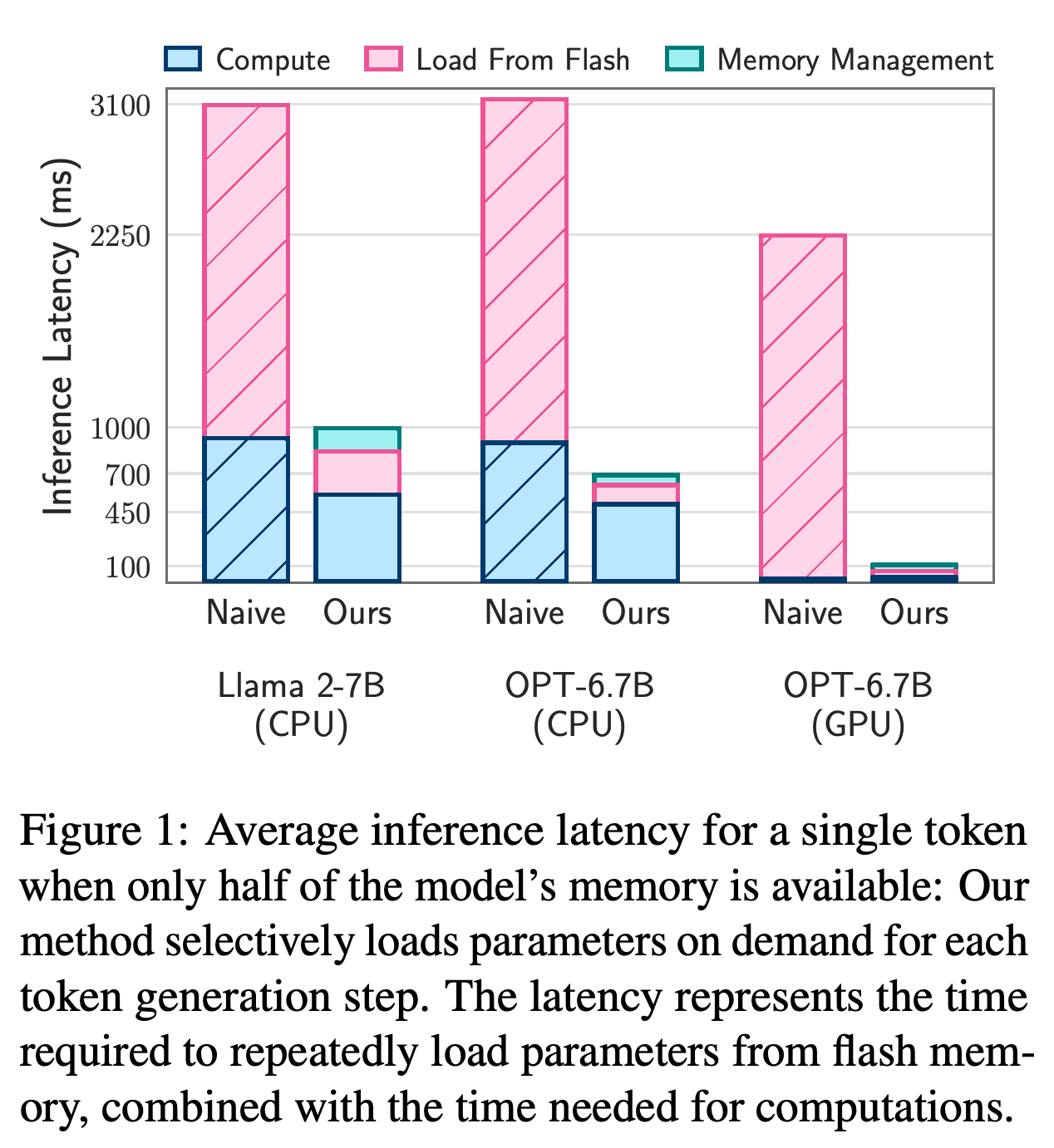
Loading every parameter into DRAM restricts the model size a device can execute: the introduction states that a 7 billion parameter model requires over 14GB for half-precision, 16-bit floating-point weights alone. The proposed alternative stores the full model in flash and brings only the required subset into DRAM during generation. Figure 1 separates computation, flash loading, and memory management to show where this approach reduces per-token latency.

Flash loading dominates the naive configurations, especially OPT-6.7B on GPU. Selective loading removes much of that cost while introducing memory-management overhead, explaining the reduction in total latency.

2 Flash Memory & LLM Inference

The hardware analysis treats storage capacity, transfer bandwidth, and read granularity—the amount fetched in each request—as constraints on inference design. Flash provides substantially more capacity than DRAM, but using that capacity efficiently requires controlling both the amount transferred and the throughput of each read.

2.1 Bandwidth and Energy Constraints

Repeatedly reading a model from flash can take seconds per forward pass and consumes more energy than moving data from DRAM into processor memory. Even a fully DRAM-resident model incurs an initial loading delay. Selective reading targets these loading costs, although this section provides no quantitative energy evaluation.

2.2 Read Throughput

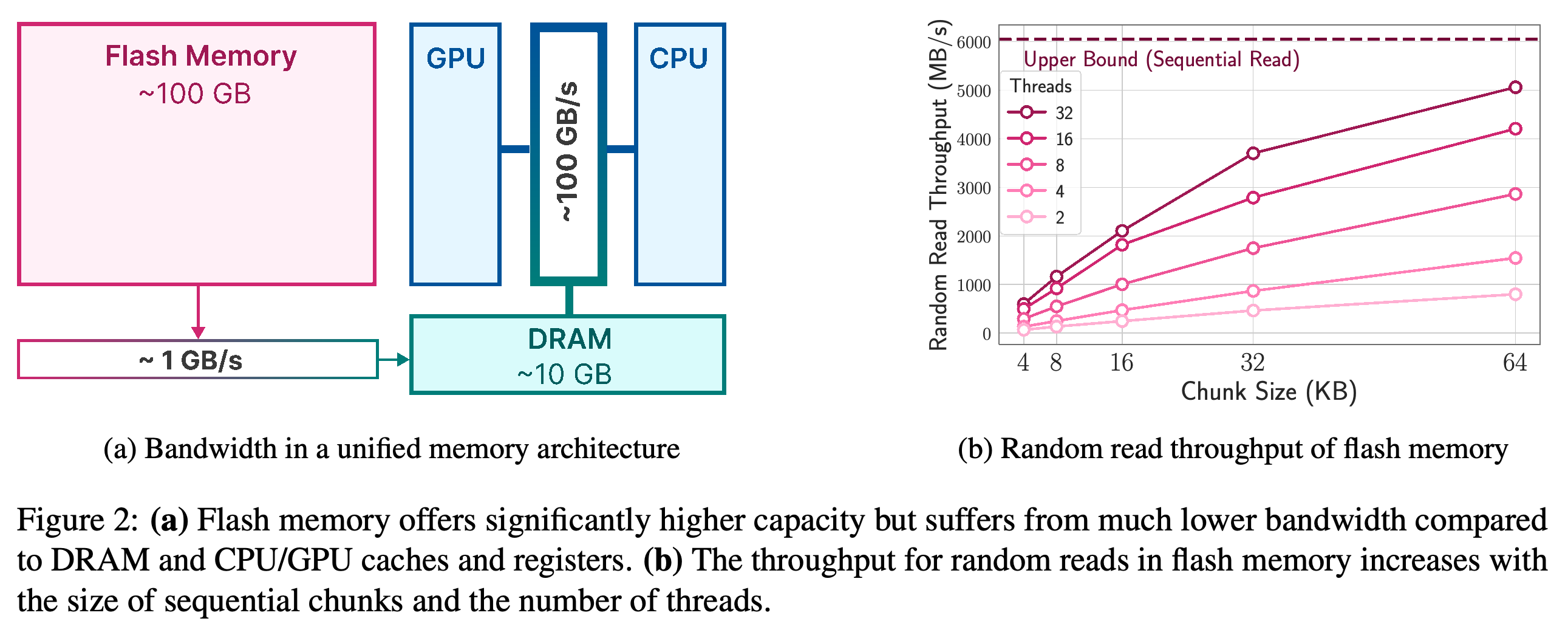
On an Apple MacBook M1 Max with 1TB flash storage, a 1GiB sequential read of an uncached file exceeds 6GiB/s. Small random reads achieve much less because operating-system, driver, and controller delays are paid repeatedly; Figure 2 shows throughput improving with both chunk size and thread count. The authors therefore advocate larger contiguous reads and parallel requests, reporting that random reads of 32KiB or larger across multiple threads can support sparse inference.

The capacity advantage of flash comes with a bandwidth penalty. The read benchmark shows that tiny random requests underuse storage bandwidth, motivating larger chunks and parallel reads.

3 Load From Flash

The loading strategy divides latency into flash input/output (I/O), memory management, and computation. Its three objectives are to transfer fewer weights, increase the size of each transferred chunk, and update resident weights without repeatedly reallocating and copying existing data. The principal optimization target is movement and management of weights.

3.1 Reducing Data Transfer

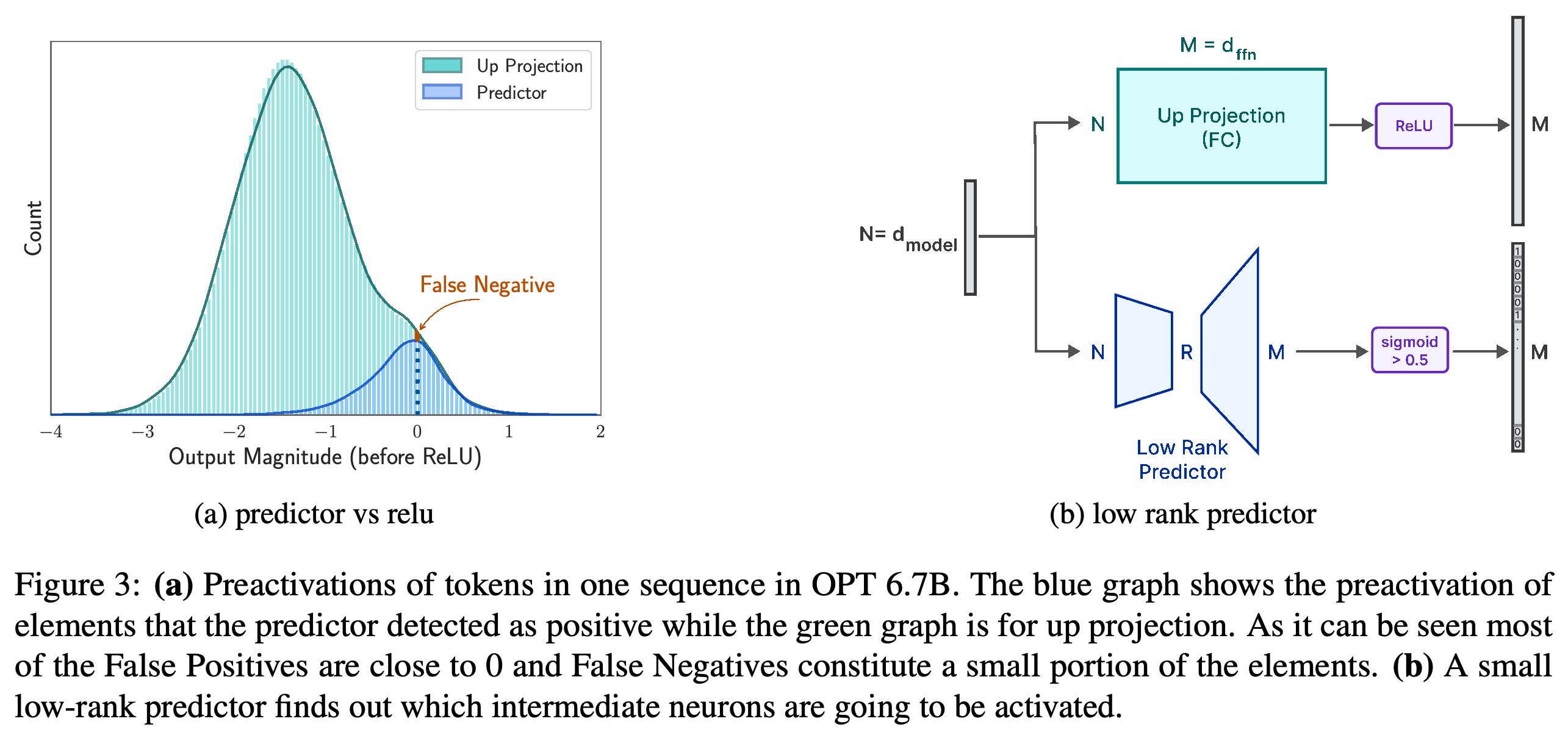
Embeddings and attention weights remain in DRAM, while FFN weights are loaded selectively; attention weights constitute approximately one-third of model size in the motivating configuration. A low-rank predictor, a compact model with an intermediate dimension smaller than its input and output dimensions, uses the current layer’s attention output to predict which neurons survive the rectified linear unit (ReLU), an activation that zeros non-positive inputs. Predictors are trained with a loss balancing positive and negative examples on 10000 samples from the C4 text dataset for 2 epochs; the paper reports 4 hours on an A100 GPU for each predictor.

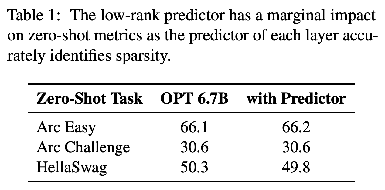
• Figure 3 illustrates prediction errors near the activation boundary: false positives select inactive neurons, while false negatives miss active neurons. Table 1 reports zero-shot scores, measured without task-specific examples, of 66.1 versus 66.2 on Arc Easy, 30.6 versus 30.6 on Arc Challenge, and 50.3 versus 49.8 on HellaSwag, comparing OPT 6.7B with its predictor-equipped version.
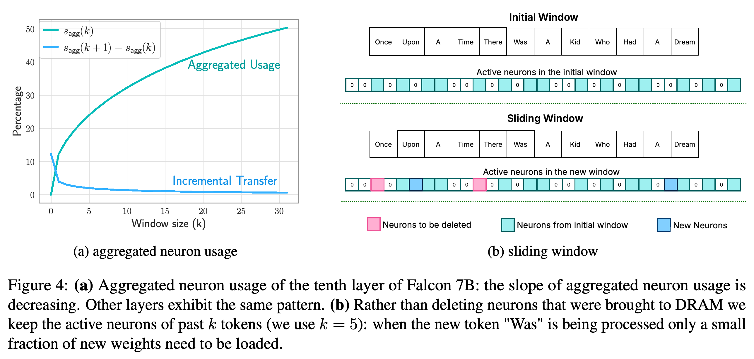
• Windowing retains weights predicted to be active for recent tokens and loads only missing weights. If s_agg(k) denotes cumulative neuron usage across k tokens, the paper expresses incremental loading as s_agg(k + 1) − s_agg(k).
• Figure 4 shows cumulative neuron usage growing with a decreasing slope. Larger windows therefore reduce fresh transfers while consuming more DRAM.

The predictor estimates which intermediate neurons will produce positive outputs before their full weights are loaded. Many selected inactive neurons have preactivations near zero, while missed active neurons form a small part of the distribution; task-score effects are measured separately in Table 1.

OPT’s predictor changes Arc Easy by +0.1 and HellaSwag by −0.5, with Arc Challenge unchanged. These three evaluations show a small score impact for OPT but do not establish accuracy preservation for every model or task.

Cumulative neuron coverage increases as more tokens enter the window, while the additional coverage required by the next token decreases. The cache update distinguishes reusable weights, expired weights, and new weights, showing how greater residency reduces fresh transfers.

3.2 Increasing Transfer Throughput

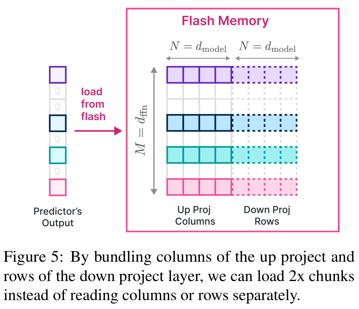
An intermediate FFN neuron requires the corresponding up-projection column and down-projection row together. Row-column bundling stores this pair contiguously, increasing each read from d_model × num_bytes to 2d_model × num_bytes, where d_model is the model’s hidden dimension and num_bytes is the storage size of one weight. Figure 5 illustrates this layout.

• A separate attempt to bundle different neurons according to co-activation, their tendency to activate together, failed: frequently active neurons appeared in many bundles and were loaded repeatedly. Strong pairwise co-activation did not make this particular storage layout effective.

Each selected intermediate neuron needs weights from both projections. Placing those weights together doubles the contiguous read size without predicting whether different neurons will activate together.

3.3 Optimized Data Management in DRAM

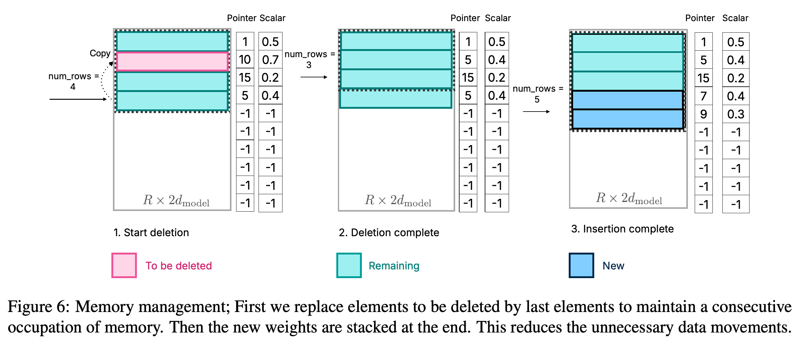
The implementation preallocates a weight matrix for each layer and tracks original neuron indices, biases, occupied rows, and recent activity. Removing a neuron replaces its row with a row from the end of the occupied region; incoming weights are appended afterward, as Figure 6 shows. This preserves contiguous occupied storage without copying the entire cache whenever its contents change.

• For c removed neurons, the stated rewrite cost is O(c × d_model), proportional to the number removed and the hidden dimension. Reordering intermediate neurons preserves the FFN output when the associated up- and down-projection weights are reordered consistently.
• The inference views use matrix[:num_rows,:d_model] for the up projection and matrix[:num_rows,d_model:].transpose() for the down projection.

Replacing an expired row with the final occupied row keeps the active region compact. New rows can then be appended without reallocating the matrix or copying all retained weights.

4 Experiments and Results

The experiments measure latency across models and execution backends, the software and hardware paths used to run inference. They include component-level loading measurements, end-to-end inference measurements, and a study of the memory-latency tradeoff; additional predictor and implementation evidence appears in the appendix.

4.1 Experimental Setup

The implementation uses HuggingFace Transformers and PyTorch, processing one sequence at a time and reserving memory for the Key-Value (KV) cache, stored attention keys and values reused during generation. Latency measurements use a small C4 validation subset, the first 128 tokens as the prompt, and 256 generated tokens. Evaluated models include OPT 6.7B, sparsified Falcon 7B, Phi-2, Persimmon 8B, and sparsified Llama 2; sparsification modifies a model to produce more zero activations.

• Hardware comprises an Apple M1 Max with a 1TB solid-state drive (SSD), an Apple M2 Ultra with a 2TB SSD, and a Linux machine with a 24GB NVIDIA RTX 4090. Apple CPU execution uses float32, a 32-bit floating-point format; Apple Metal GPU execution uses float16, a 16-bit format; and RTX execution uses bfloat16, another 16-bit format.
• Most configurations allocate approximately 50% of model size to resident weights; Phi-2 uses 65% because it has less activation sparsity. The experiments impose constrained allocations on the tested machines and reserve separate capacity for the KV cache.
• The naive baseline loads weights on demand during each forward pass. The hybrid baseline retains part of the model and streams the remainder without exploiting sparsity; baseline I/O times use optimistic theoretical transfer rates. Reads use 32 threads, and operating-system caching is disabled for storage benchmarking.

4.2 Faster Load From Flash

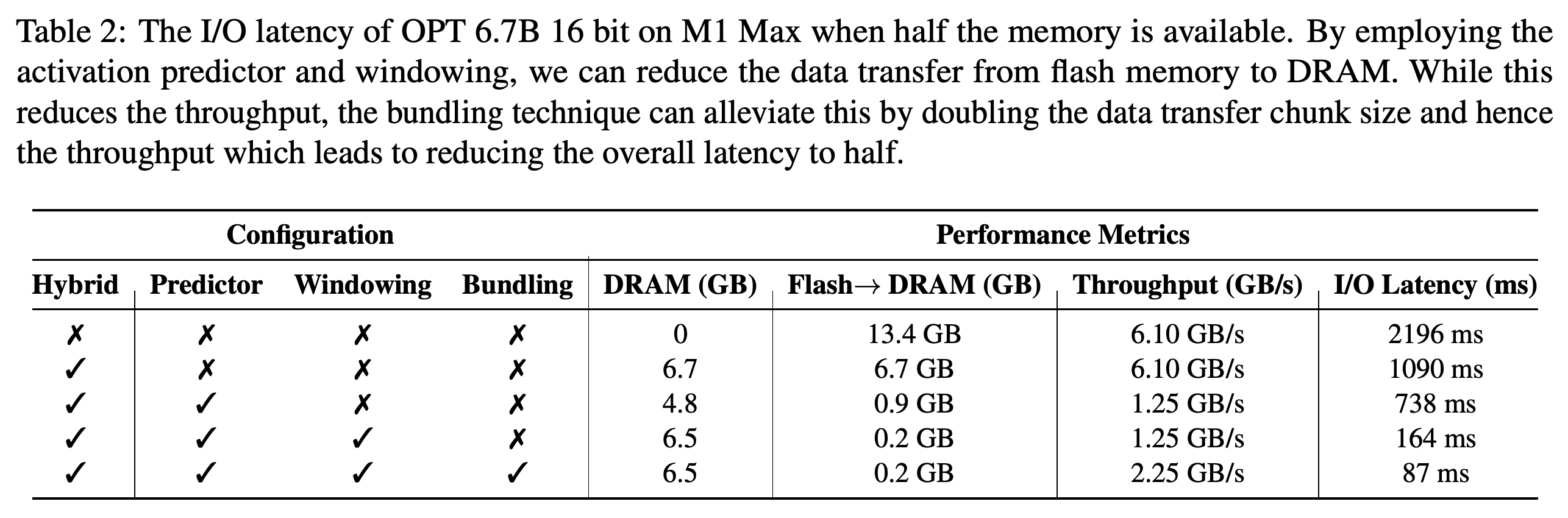
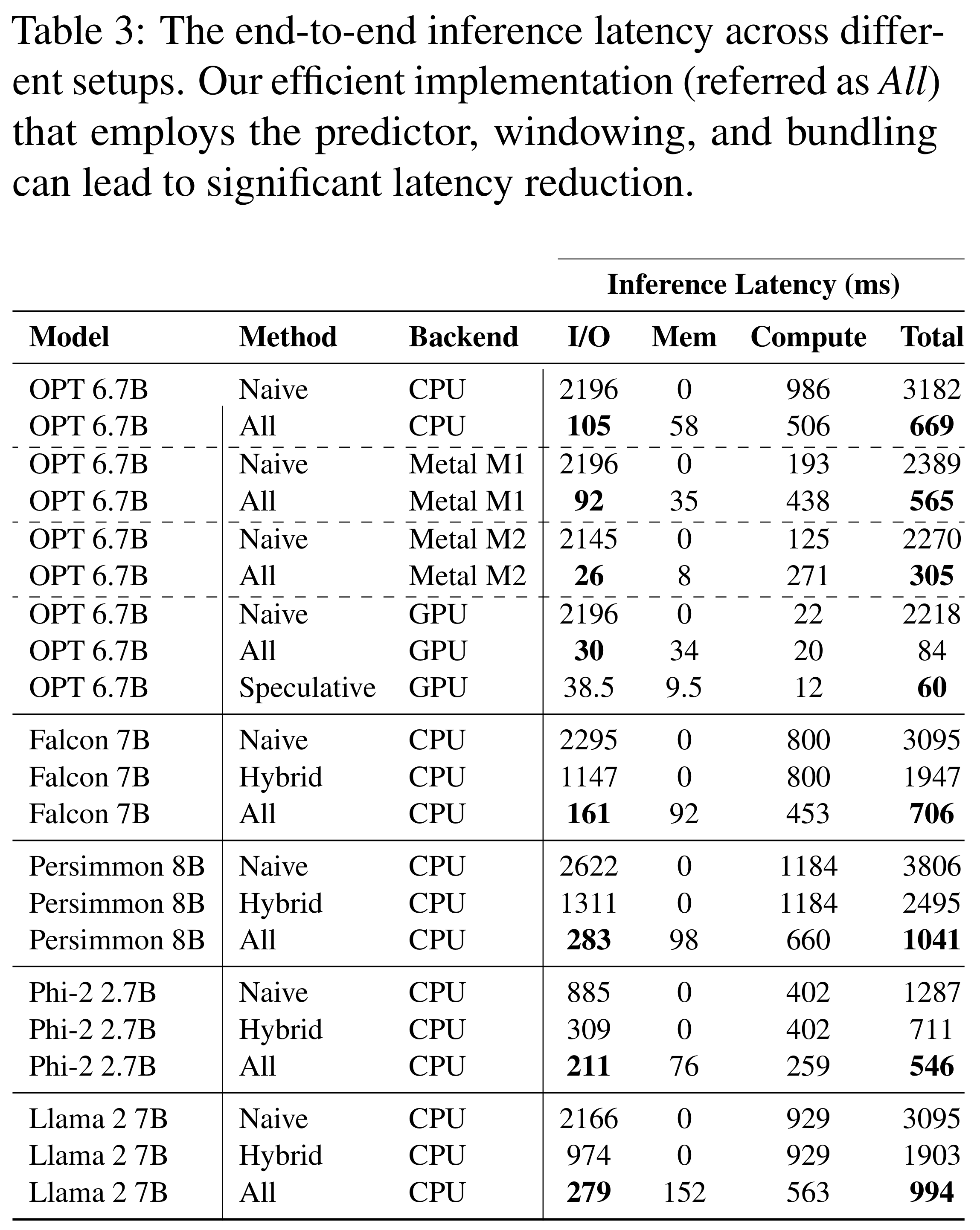
Table 2 isolates the effect of each loading technique for 16-bit OPT 6.7B on M1 Max: prediction and windowing reduce transferred data, while bundling improves throughput for the remaining sparse reads. Table 3 reports end-to-end OPT 6.7B latency reductions from 3182 to 669ms on CPU, 2389 to 565ms on Metal M1, 2270 to 305ms on Metal M2, and 2218 to 84ms on the NVIDIA GPU.

• In Table 2, hybrid loading transfers 6.7GB at 1090ms; adding prediction reduces transfer to 0.9GB at 738ms. Windowing reduces it to 0.2GB at 164ms, and bundling increases throughput from 1.25 to 2.25GB/s, reducing I/O latency to 87ms.
• CPU end-to-end latencies for the complete method are 706ms for Falcon 7B, 1041ms for Persimmon 8B, 546ms for Phi-2 2.7B, and 994ms for Llama 2 7B. Their respective hybrid baselines are 1947, 2495, 711, and 1903ms.
• Sparse execution can introduce compute overhead: OPT 6.7B compute time on Metal M1 rises from 193 to 438ms, even while total latency falls. In this configuration, the loading savings outweigh the additional computation.

The ablation distinguishes transfer volume from throughput: prediction and windowing reduce bytes, while bundling raises throughput from 1.25 to 2.25GB/s for the same reported 0.2GB transfer. I/O latency consequently falls from 164 to 87ms.

End-to-end improvements occur across the listed models, with substantially different magnitudes. The breakdown also reveals increased compute time on the Metal backends and a further GPU reduction from 84 to 60ms with speculative decoding.

4.3 The Memory-Latency Tradeoff

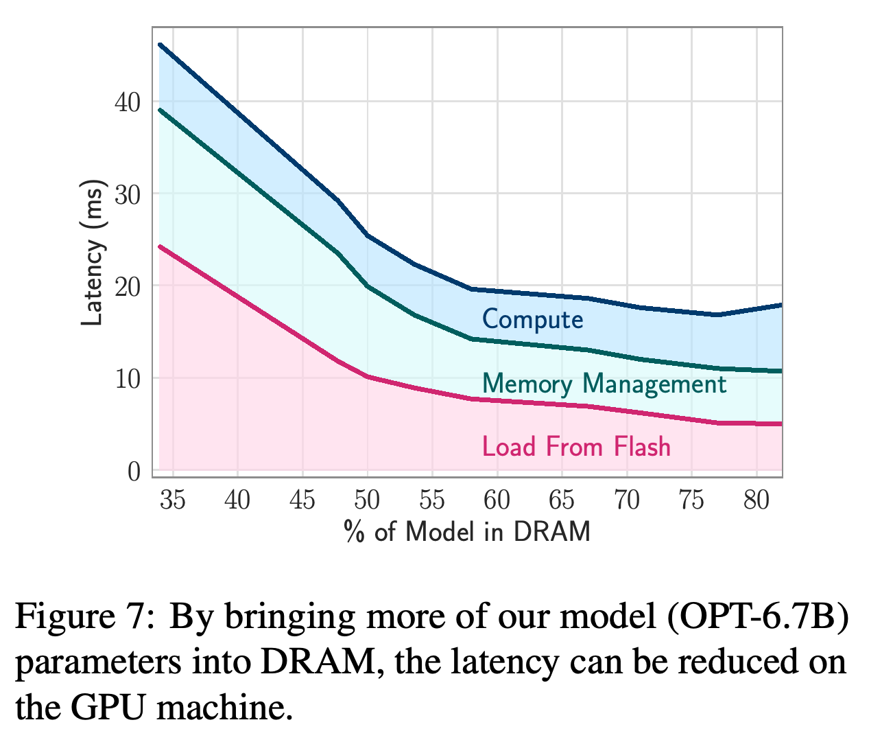
Increasing the window retains more weights in DRAM and reduces the number fetched for subsequent tokens. Figure 7 demonstrates this tradeoff for OPT-6.7B on the GPU machine, with lower total latency as the resident fraction increases across most of the plotted range. Approximately half-model residency is an experimental operating point rather than a fixed requirement.

Keeping a larger fraction of OPT-6.7B resident reduces flash-loading and memory-management latency across most of the range. The total curve shows diminishing gains and a slight rise at the highest plotted residency, so the measured relationship is not strictly monotonic.

5 Ablation analysis

The ablations test longer generation and the addition of speculative decoding, where a larger model verifies tokens proposed by a draft model. A separate power discussion distinguishes instantaneous power from the total energy consumed during generation.

5.1 The Impact of Longer Generation

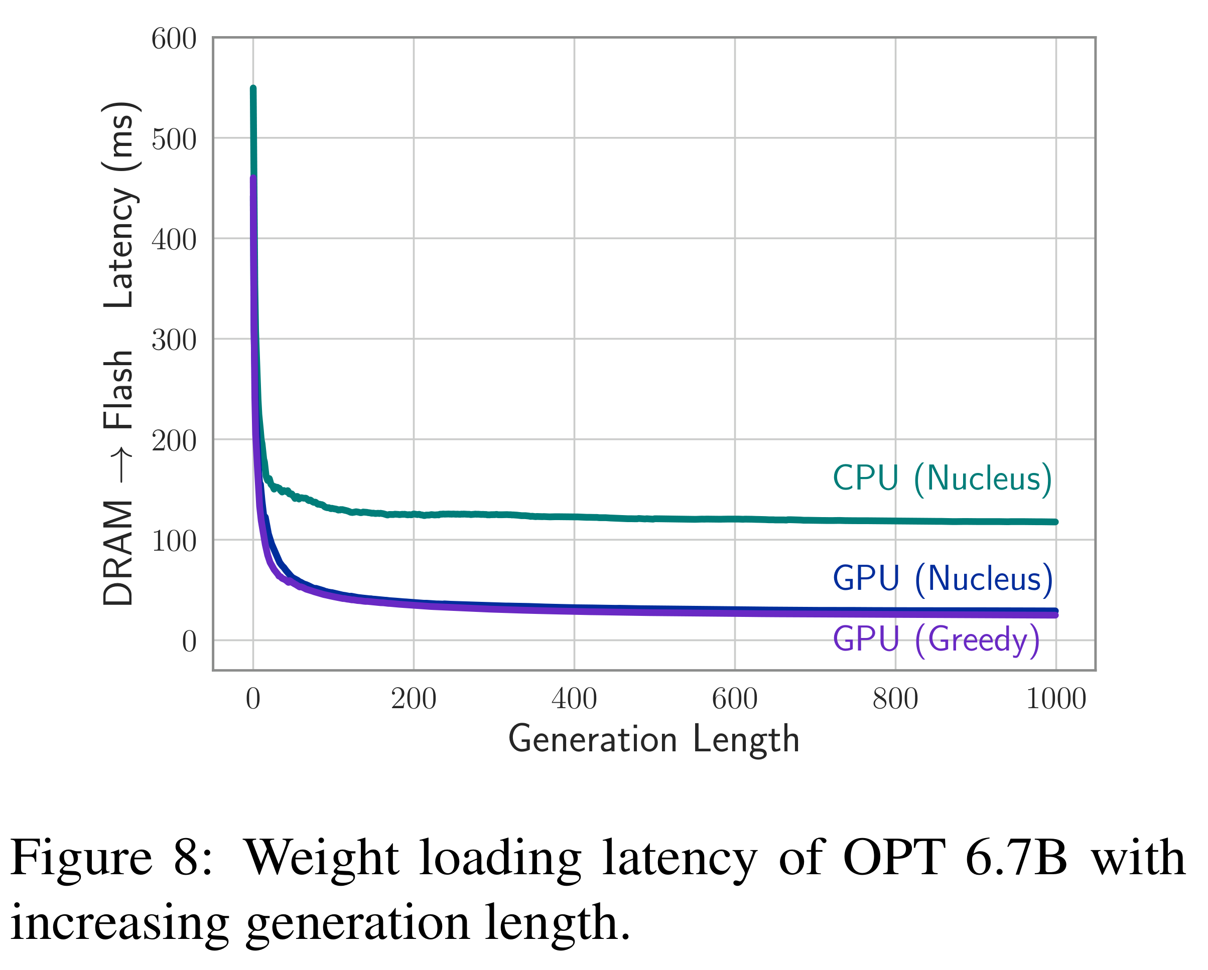
For OPT 6.7B, the authors extend generation from 256 to 1000 tokens and report no increase in average flash-loading latency over that interval. Figure 8 shows a large initial loading cost followed by declining and then approximately stable average latency as the weight cache fills. Nucleus sampling, a non-greedy token-selection method, also preserves the observed loading performance on CPU and GPU.

Average loading latency falls sharply after the initial cache fill and remains approximately stable through 1000 generated tokens. This supports sustained loading performance over the measured interval; the figure contains no direct temperature measurements.

5.2 Speculative Decoding

Speculative decoding requires choosing which proposed tokens’ neurons to retain before acceptance is known; rejected proposals can otherwise occupy cache space without supporting the next step. With \(\lambda=4\) draft tokens, the paper reports a further 1.4× decoding speedup, with Table 5 giving 84.64 ± 6.16ms for the complete GPU method and 60.16 ± 13.4ms with speculation, where ± denotes standard deviation.

• The proposed cache rule retains k tokens ending at the \(\alpha(\lambda+1)\)th token, where α is the acceptance ratio. The authors describe its optimality as a conjecture.

5.3 A Note on Power Consumption

Compared with a dense model of similar size, which does not exploit activation sparsity, the sparse approach draws less instantaneous power but takes longer to generate tokens, producing higher total energy consumption in the authors’ comparison. The paper supplies no numerical power traces and leaves systematic quantitative evaluation to future work. Its latency gains over flash-loading baselines therefore do not establish energy savings over dense execution.

6 Related Works

The paper positions flash-efficient loading alongside compression and selective computation. Deja vu predicts activation sparsity to select weights from GPU memory, while FlexGen moves weights and the KV cache among GPU memory, DRAM, and flash. This work concentrates on the case where the full model cannot remain in available working memory and repeated flash access becomes a central cost.

7 Discussion

The discussion attributes the gains to combining reuse across recent tokens, contiguous paired-weight reads, and efficient management of resident weights. It reports approximately 4–5× CPU and 20–25× GPU acceleration for OPT relative to traditional loading methods, while Table 3 provides the explicit backend-specific measurements. Improved bundling, data structures, and hardware-specific execution are presented as future work.

8 Limitations

The evidence is limited to single-sequence inference, with preliminary speculative decoding results and predominantly half-model memory allocations. Prompt processing, multiple concurrent sequences, broader memory budgets, systematic thermal behavior, and quantitative energy evaluation require further study. The demonstrated method depends on sparse or sparsified networks; adapting the concept to non-sparse models remains a proposed direction.

Appendix

• A Appendix Overview maps the supplementary evidence: predictor accuracy and efficiency in B, implementation and model-specific results in C, the failed co-activation bundling experiment in D, extended related work in E, implications for smaller devices in F, and generated-text comparisons in G.
• B Low-Rank Activation Predictor: Additional Results evaluates the predictor’s effect on accuracy, transferred weights, and inference overhead. Avoiding missed active neurons requires predicting extra neurons, which adds redundant flash reads.
• B.1 Sparsity patterns of predictors uses 100 random C4 validation samples. Predictors select approximately 3× the actually active neuron count for OPT and Persimmon and approximately 2× for Phi-2, accepting redundant loads to reduce missed activations. Later layers are more active in OPT and Persimmon, while middle layers are more active in Phi-2.
• B.2 Accuracy of models using predictors shows that accuracy preservation depends on predictor rank and threshold. On Massive Multitask Language Understanding (MMLU), a benchmark of accuracy across tasks, larger predictors in Persimmon’s last 4 layers preserve performance better than rank-256 predictors throughout. Phi-2 falls from 54.3 after ReLU conversion with distillation to 52 with predictors, and Table 4 also shows model-dependent changes in zero-shot scores.
• B.3 Overhead of predictors reports an average OPT-6.7B predictor rank of 240 and less than 2.4% of non-embedding weights and floating-point operations (FLOPs), an arithmetic-operation count. Measured inference-time shares are 2.75% on M1 Max CPU and 4.8% on RTX GPU for OPT, 2.85% on CPU for Persimmon, and 3.92% on CPU for Llama 2. Falcon predictors account for 4% of model size and CPU computation.
• C Extended Results describes implementation changes for handling changing sparse weight shapes efficiently. On macOS 14.3, custom Metal kernels, GPU computation routines borrowed from Apple’s MLX framework, handle dynamic shapes within a binary extension; MTLStorageModeShared allows CPU and GPU access to shared buffers. Storage measurements disable filesystem caching with F_NOCACHE through fcntl() on macOS and iOS and DirectIO on Linux; macOS benchmarks additionally clear resident buffers using purge.
• C.1 Results for OPT 6.7B Model uses rank-128 predictors in the first 28 layers and rank-1024 predictors in the last 4, reporting average false-negative and false-positive rates of 5% and 7%. The stated resident-weight breakdown is 1.25% predictors, 3% embeddings, 32.3% attention, and 15.5% cached FFN weights, totaling 52.1% of model size. The text describes k = 4 but also refers to the past 5 tokens, leaving the window-count convention ambiguous; Table 5 reports CPU latency of 669.20 ± 39.74ms per token.
• C.2 Results for Falcon 7B Model uses a ReLU-converted, fine-tuned model, with predictor ranks of 256 in the first 28 layers and 1152 in the last 4. A 4-token window retains 33% of FFN weights and yields a total resident fraction of 52.93% of model size. Approximately 161ms of flash loading and 90ms of memory management describe memory-related costs; Table 3’s 706ms total also includes computation.
• C.3 Persimmon 8B uses its existing squared-ReLU activation, which squares the positive ReLU output, without further model fine-tuning. Predictors have rank 256 in the first 32 layers and 1152 in the last 4, with threshold 0.7; a nominal 4-token window shrinks when cached weights exceed 25% of FFN size. Table 5 reports 1090.08 ± 79.08ms total CPU latency, differing from Table 3’s 1041ms, without an explicit reconciliation.
• C.4 Phi-2 first converts the model to ReLU and fine-tunes it on refined-web data with a distillation loss, a training term used to recover model quality. MMLU decreases from 57 to 54.3 after this conversion and to 52 after predictor integration. The implementation assigns larger predictors to less-sparse middle layers, adjusts the window to a 65% memory budget, and reports approximately 2.35× acceleration over naive loading.
• C.5 Llama 2 evaluates a sparsified model using FATReLU, a thresholded activation that retains neurons with sufficiently large gated values. It uses a 2-token window, rank-1024 predictors in 4 middle layers, rank-256 predictors elsewhere, and stops caching additional weights above 55% of model size. Reported MMLU scores are 41.8 for the original model, 38.96 for the sparsified model, and 38.63 with predictors; directly retaining the gate projection, which determines sparse activations, instead requires 65% residency even with a window of 1.
• D Bundling Based on Co-activation examines whether neurons that frequently activate together should share storage bundles. Despite strong co-activation with each neuron’s most frequent partner, bundling those pairs repeatedly loads popular neurons because many neurons share the same partner. The experiment supplies a negative result for this particular layout.
• E Extended Related Works expands the comparison with compression, selective loading, hardware optimizations, speculative execution, and Mixture of Experts, architectures that select among separate FFN components. The authors present these approaches as complementary to reducing flash traffic and arranging weights for efficient flash reads.
• F Small Device Implications proposes combining the method with quantization, storing weights at reduced numerical precision, to reduce a 7B model’s residency from a 3.5GB dense baseline to less than 2GB using 4-bit weights. Across 100 sequences, the reported average active-neuron percentages for OPT 6.7B and its quantized version are 3.30% and 3.27%, supporting similar sparsity in that comparison. Smartphone execution with specialized 4-bit kernels is outside the implementation scope, so the memory estimate is not an end-to-end device demonstration.
• G Qualitative Evaluations compares original and predictor-equipped model continuations for “Once upon a time there was a” and a C4 passage. Tables 7–9 show readable but differing outputs, including repetition and incomplete continuations. These selected examples illustrate behavior but provide no systematic estimate of generation quality or failure frequency.

Brief Thoughts

The component-level ablation gives the clearest account of the gains: prediction and windowing reduce transferred bytes, bundling recovers read throughput, and preallocation limits cache-copy overhead. Practical comparisons should include the hybrid baseline and model-specific accuracy results, because the largest headline gains use naive loading and some models lose accuracy during sparsification and prediction. The experiments establish a capacity-latency tradeoff under constrained memory allocations; smartphone performance and energy efficiency still require direct evaluation.