


MoBluRF: Motion Deblurring Neural Radiance Fields for Blurry Monocular Video | Summary
21 Dec 2023 | Paper Review Neural Radiance Fields Motion Deblurring Novel View SynthesisContents
This article explains the key points of MoBluRF: Motion Deblurring Neural Radiance Fields for Blurry Monocular Video.
- 2023-12-21 (arXiv)
- Bui, Minh-Quan Viet, Park, Jongmin, Oh, Jihyong, Kim, Munchurl.
- School of Electrical Engineering, Korea Advanced Institute of Science and Technology, Department of Imaging Science, GSAIM, Chung-Ang University
- Paper
Summary
- MoBluRF reconstructs sharp images at new viewpoints and times from a single-camera video blurred by camera and object motion. On the seven-sequence Blurry iPhone benchmark, its average co-visibility-masked peak signal-to-noise ratio, a reconstruction measure excluding test regions unseen during training, is 17.33 versus 16.22 for GShiftNet + T-NeRF, a video-deblurring and dynamic-scene reconstruction cascade; MoBluRF uses synthesized inaccurate camera poses, while the cascade receives the original poses.
- The method learns a neural radiance field (NeRF), a neural representation of scene color and density, in two stages: Base Ray Initialization (BRI) refines viewing rays derived from inaccurate camera poses, and Motion Decomposition-based Deblurring (MDD) predicts hidden sharp rays whose rendered colors are averaged to reproduce blur. Separate losses encourage static/dynamic scene decomposition without motion-mask supervision and regularize geometry using pretrained single-image depth estimates.
- On Stereo Blur, MoBluRF improves average peak signal-to-noise ratio from DyBluRF’s 25.14 to 25.69 and reduces learned perceptual image patch similarity, a perceptual distance measure, from 0.082 to 0.078. Rendering takes 9.1 seconds per 480 × 360 frame on one RTX 3090 Ti, and the paper documents appearance errors under imbalanced training illumination.
I. Introduction
Novel view synthesis (NVS), the generation of images from new camera viewpoints and times, becomes difficult when exposure integrates camera shake and moving objects into blurred observations. MoBluRF: Motion Deblurring Neural Radiance Fields for Blurry Monocular Video targets three coupled problems: maintaining consistent three-dimensional geometry during deblurring, representing both camera and object motion, and preventing inaccurate camera positions and orientations from destabilizing reconstruction.
- Deblurring individual frames before reconstruction can introduce inconsistencies across views that the subsequent scene model cannot repair.
- The paper contributes a two-stage optimization procedure, blur modeling through hidden sharp rays, two regularizers, and a synthesized Blurry iPhone evaluation dataset.
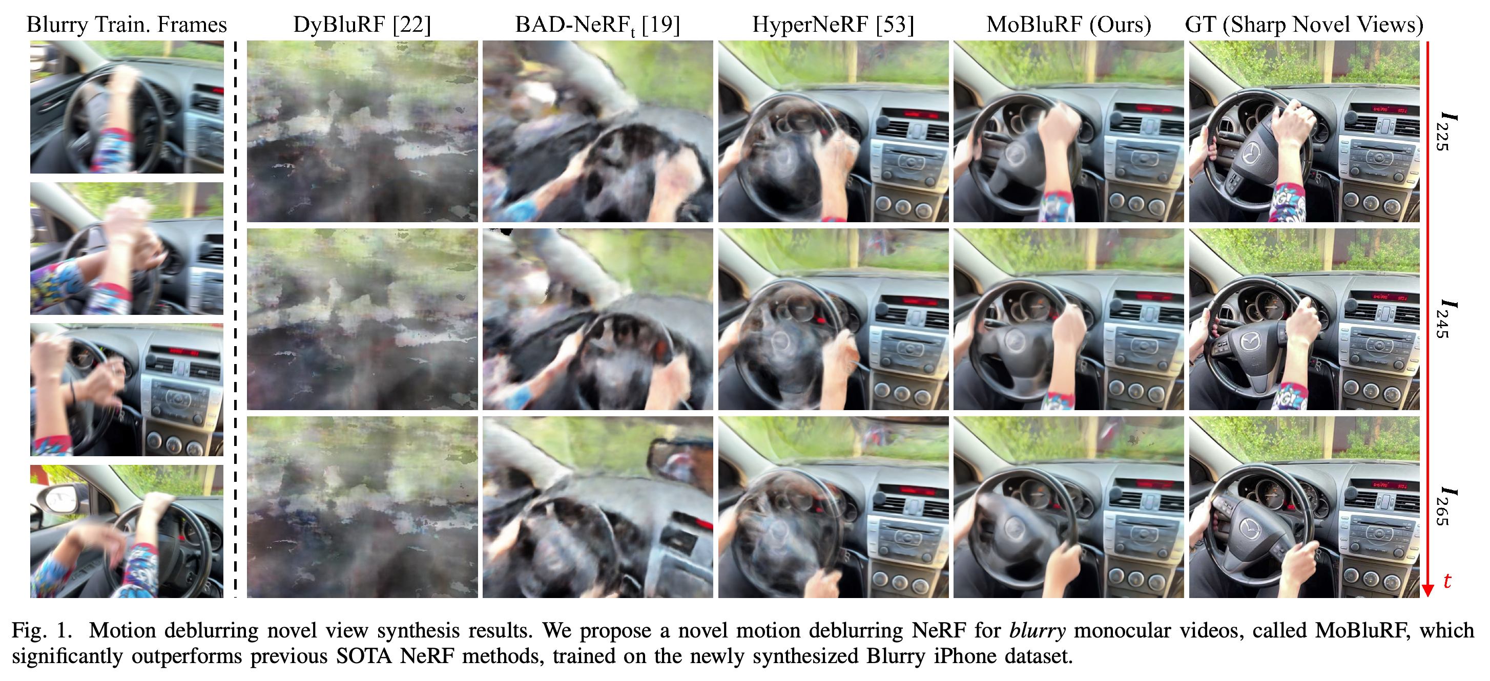
The steering-wheel sequence combines moving hands with changing camera views. MoBluRF preserves more coherent hand and dashboard structure than the displayed alternatives, providing qualitative support without establishing a numerical margin.
II. Related Work
The related work distinguishes dynamic-scene reconstruction from methods that explicitly model blurred observations. These strands motivate combining a time-dependent scene representation with motion-aware deblurring and a separate initialization stage.
A. NVS for Dynamic Scenes
Dynamic-scene methods represent motion through scene flow, which describes three-dimensional point movement, canonical fields, which map observations to a shared reference space, or directly time-dependent radiance fields. Other methods use Gaussian Splatting, which renders a scene represented by spatial Gaussian elements; the paper argues that these approaches need an additional blur model to reconstruct sharp scenes from blurred inputs.
- NSFF, DynamicNeRF, and DynIBaR combine static and dynamic scene representations with motion or geometry constraints.
- T-NeRF, HyperNeRF, and TiNeuVox learn transformations from observation space to a canonical space, while Gaussian-based methods model time-varying scene attributes.
B. Deblurring NVS
Static deblurring methods estimate blur kernels, which describe how sharp observations are combined, or camera trajectories during exposure, but their original formulations do not address deforming scenes in monocular video. DyBluRF averages sharp renderings over exposure and models object trajectories; the authors identify direct trajectory estimation from inaccurate poses and reliance on external motion masks, depths, and optical flow, the apparent movement between images, as weaknesses in their longer, more complex sequences.
- MoBluRF initializes reference viewing rays before deblurring and learns its motion masks internally.
- Its geometry regularizer still uses pretrained depth estimates, so removing motion-mask supervision does not remove all external priors.
III. Proposed Method: MoBluRF
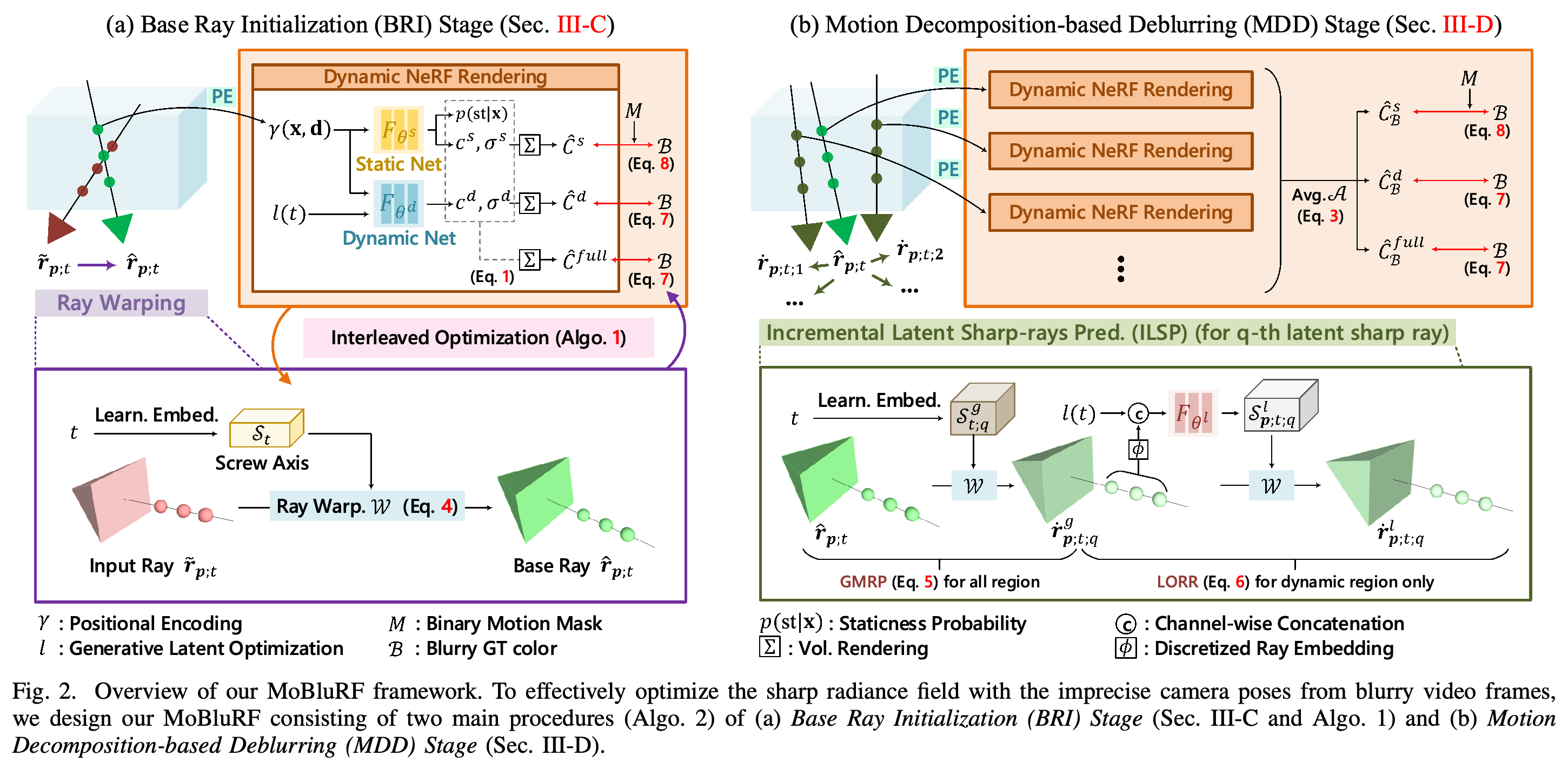
MoBluRF first reconstructs a coarse dynamic scene while correcting input rays, then learns a blur-aware sharp scene from the initialized rays. Figure 2 and Algorithms 1–3 distinguish initialization, blur-aware training, and sharp-view inference.
BRI corrects a reference ray while reconstructing the scene, and MDD expands that ray into exposure contributions. The dynamic-region branch identifies where local refinement follows global prediction.
A. Design Considerations
A base ray is the reference viewing ray from which the model predicts latent sharp rays, the hidden rays whose renderings contribute to an observed blurred pixel. If base rays inherit inaccurate camera poses, the dynamic network can explain pose errors as object deformation, producing incorrect geometry and exposure trajectories.
- BRI uses static-scene cues to improve base-ray initialization before introducing the blur model.
- MDD subsequently predicts global motion and local object-motion corrections from these initialized rays.
B. Preliminaries
The Static Net predicts color, density, and the probability that a three-dimensional point is static; the Dynamic Net also receives a learned time embedding, a numerical representation indexed by time, and predicts time-dependent color and density. Probabilistic volume rendering, the accumulation of color along a ray using density-dependent weights, combines these networks into the full image.
- A binary motion mask is obtained by thresholding the accumulated dynamic probability along each ray at greater than 0.5.
- Equation (3) models a blurred pixel by uniformly averaging the base-ray rendering and the renderings of Nb latent sharp rays, giving Nb + 1 contributions.
- The blur model operates during training; inference renders one sharp target ray per pixel.
C. Base Ray Initialization (BRI) Stage
BRI warps input rays through a learned six-dimensional screw axis, a rotation-and-translation parameterization, indexed by frame time. Its interleaved optimization alternates pose-related and dynamic-network updates to reduce the tendency to absorb pose errors into apparent object deformation.
- At even iteration indices, the method updates the Static Net and ray-warping parameters using the static-region photometric loss, which measures rendered-color error.
- At odd iteration indices, it updates both scene networks while holding the ray-warping parameters fixed.
- BRI runs for 2 × 10^5 iterations; its learned base-ray correction is frozen during MDD.
D. Motion Decomposition-based Deblurring (MDD) Stage
MDD uses Incremental Latent Sharp-rays Prediction (ILSP), a global-then-local procedure for estimating exposure-related rays. Global Motion-aware Ray Prediction (GMRP) applies learned time-dependent transformations to generate multiple rays for all scene regions, and Local Object-motion-aware Ray Refinement (LORR) adds pixel-dependent corrections only in predicted dynamic regions.
- GMRP maps each initialized base ray to Nb latent rays and accounts for camera and object motion at a global level.
- LORR uses a multilayer perceptron (MLP), a feedforward neural network, to predict an additional screw-axis transformation from a discretized ray embedding, a representation sampled along the ray, and the time embedding.
- Static regions use the globally predicted rays; dynamic regions use the locally refined rays. Their rendered colors are averaged with the base-ray color and compared with the blurred input.
E. Loss Functions
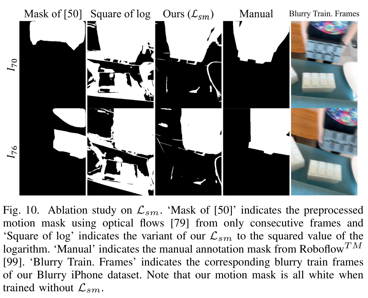
Photometric losses compare rendered and observed colors using squared error; the static-network loss excludes predicted dynamic regions. Unsupervised Staticness Maximization penalizes the absolute logarithm of staticness probability, countering the collapse in which the dynamic network explains the entire scene.
- Local Geometry Variance Distillation compares normalized cross-products of local three-dimensional geometry derivatives obtained from rendered and pretrained depth estimates.
- The authors motivate differentiation and normalization as ways to handle depth shift and scale ambiguities, respectively, and compare this regularizer with a conventional depth loss.
- The depth prior comes from pretrained DPT, the single-image depth estimator cited by the paper; it supplies auxiliary supervision rather than measured scene depth.
IV. Experiments
Implementation Details. MoBluRF uses the JAX numerical-computing framework and the Dycheck scene-reconstruction codebase, with 128 samples per cast ray, 2 × 10^5 BRI iterations, and 1 × 10^5 MDD iterations. The default uses Nb = 6 latent sharp rays, geometry-loss weight 0.075, staticness-loss weight 0.002, and the Adam optimizer with exponential learning-rate schedules.
- Screw-axis embedding learning rates range from 10^-4 to 10^-6; the remaining neural-network learning rates range from 10^-3 to 10^-4.
- The trunk, density, and color networks have 9, 1, and 2 layers, respectively; trunk and color hidden dimensions are 256 and 128.
- The local object-motion network has 8 layers of width 128. Position and viewing-direction encodings use 8 and 4 frequencies, the time embedding has dimension 8, and the discretized ray embedding uses 32 samples.
1) Blurry iPhone Dataset: The authors synthesize blurred observations from seven iPhone sequences averaging 365 frames each. Video frame interpolation, which generates intermediate frames, increases the frame rate by 8× before averaging interpolated frames with the original center frame; original sharp frames and camera poses support evaluation.
- Training camera poses are also synthesized: rotations use quaternion spherical linear interpolation, which interpolates orientations, followed by averaging; translations use linear interpolation and averaging.
- These synthesized poses differ from the original center-frame poses, introducing a controlled pose-initialization challenge alongside image blur.
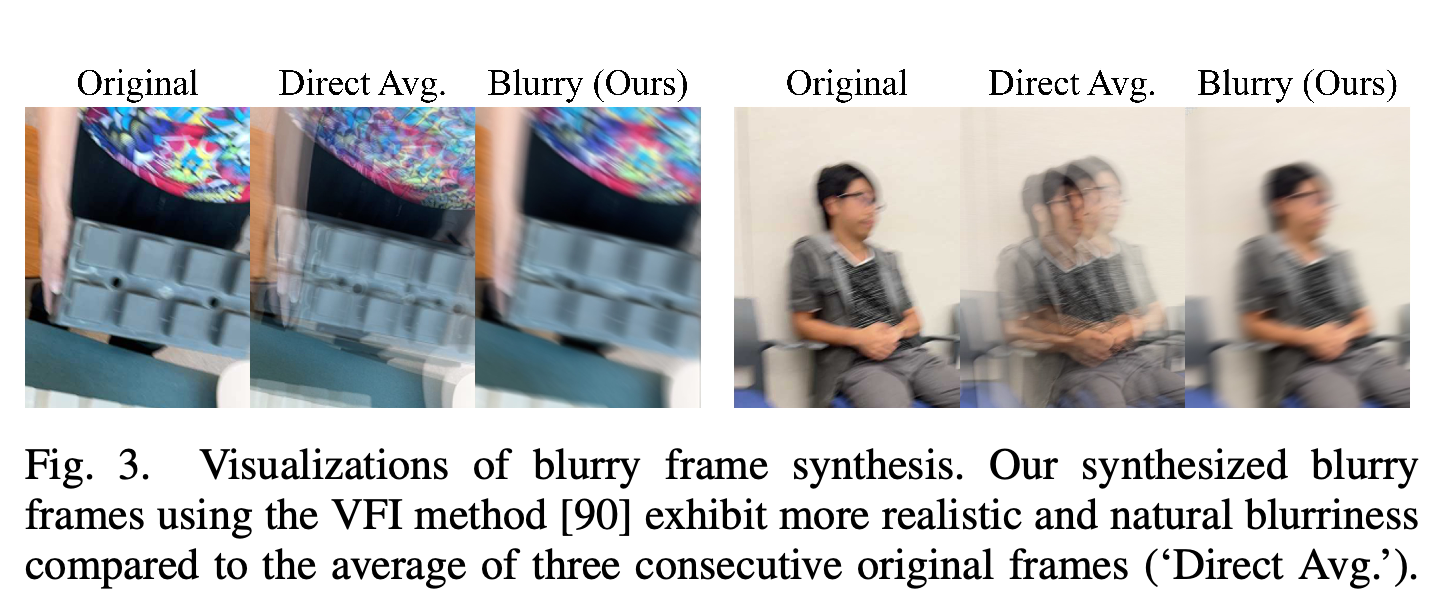
- Figure 3 compares this synthesis with direct averaging of three original consecutive frames.
Direct averaging leaves separated appearances of moving content, whereas interpolation-based averaging produces smoother motion trails. The examples support the synthesis choice but do not establish equivalence to physical camera exposure.
2) Stereo Blur Dataset: Six scenes provide blurred left-view videos and corresponding sharp right-view videos. The source videos were captured at 60 fps, interpolated to 480 fps, and averaged to generate blur; the experiments extract 24 frames per scene and estimate camera parameters using COLMAP, a camera-reconstruction system.
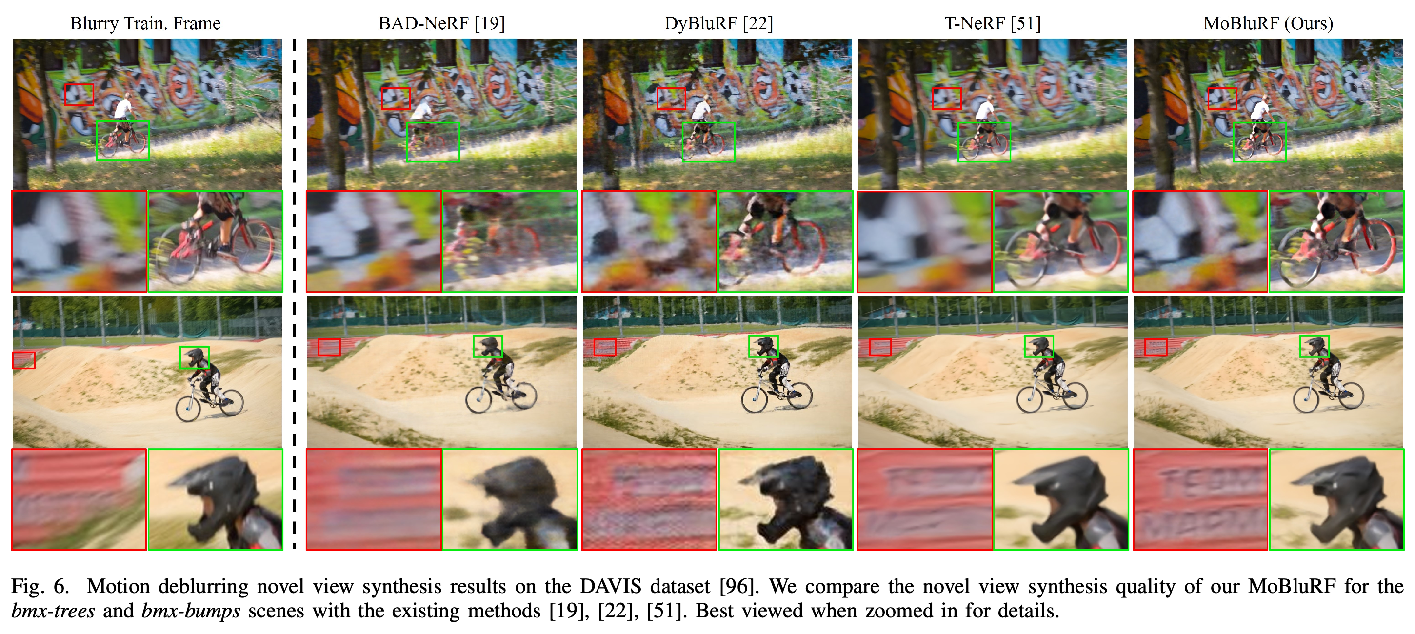
3) DAVIS Dataset: In-the-wild monocular sequences averaging 69.7 frames per scene provide qualitative tests with real motion blur; camera parameters follow the strategy in reference [69] because COLMAP does not produce reasonable poses for this setting. Evaluation uses masked image metrics on Blurry iPhone, unmasked image metrics on Stereo Blur, and tOF, a temporal optical-flow measure of consistency between reconstructed frames.
- The masked metrics exclude test regions unseen during training: mPSNR measures peak signal-to-noise ratio, mSSIM measures structural similarity, and mLPIPS measures learned perceptual image patch similarity.
- Higher PSNR and SSIM are better; lower LPIPS and tOF are better.
- DAVIS evidence is visual rather than a quantitative benchmark table in this PDF.
A. Experimental Results
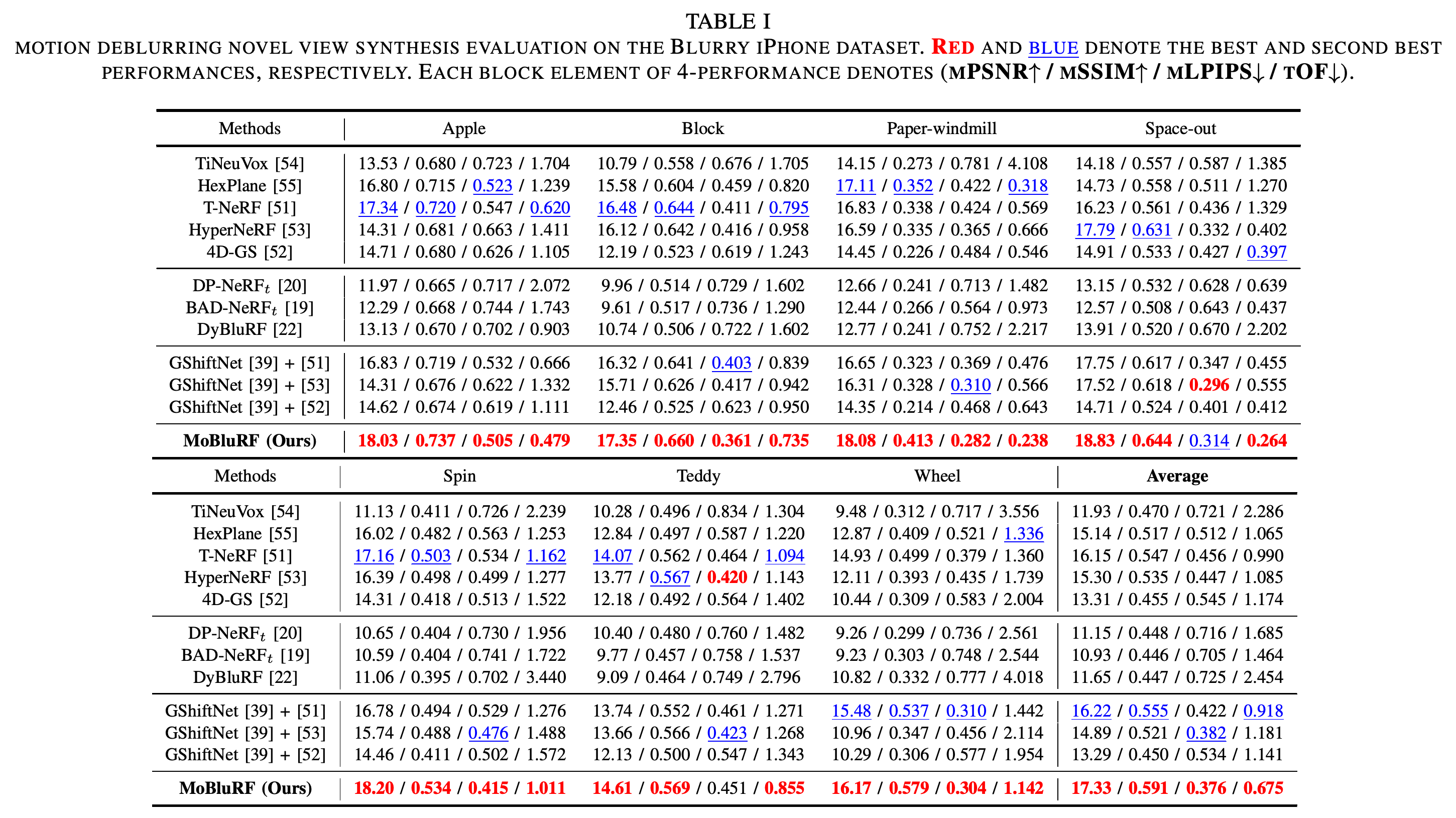
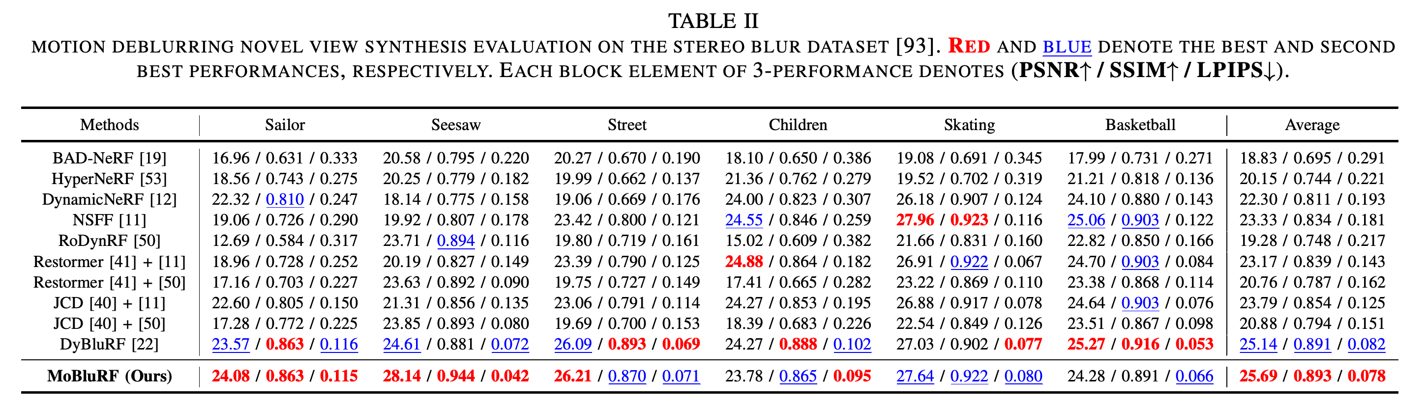
1) Motion Deblurring Novel View Synthesis: Table I reports Blurry iPhone averages of 17.33 / 0.591 / 0.376 / 0.675 for mPSNR / mSSIM / mLPIPS / tOF, the best averages among the listed methods. Table II reports Stereo Blur averages of 25.69 / 0.893 / 0.078 for PSNR / SSIM / LPIPS, compared with DyBluRF’s 25.14 / 0.891 / 0.082.
- Static deblurring baselines BAD-NeRF and DP-NeRF receive time embeddings for the Blurry iPhone comparison, yielding BAD-NeRFt and DP-NeRFt.
- GShiftNet preprocessing cascades use the original camera poses rather than synthesized inaccurate poses. GShiftNet + T-NeRF reaches 16.22 / 0.555 / 0.422 / 0.918, the best competing averages for mPSNR, mSSIM, and tOF; GShiftNet + HyperNeRF has the best competing average mLPIPS, 0.382.
- Best dataset averages do not imply uniformly best scene results: on Stereo Blur, MoBluRF trails DyBluRF in Children PSNR and SSIM and Basketball PSNR, SSIM, and LPIPS.
MoBluRF leads all four dataset-average metrics at 17.33 / 0.591 / 0.376 / 0.675. Individual scenes contain exceptions, including better perceptual distance for GShiftNet + HyperNeRF on Space-out and HyperNeRF on Teddy.
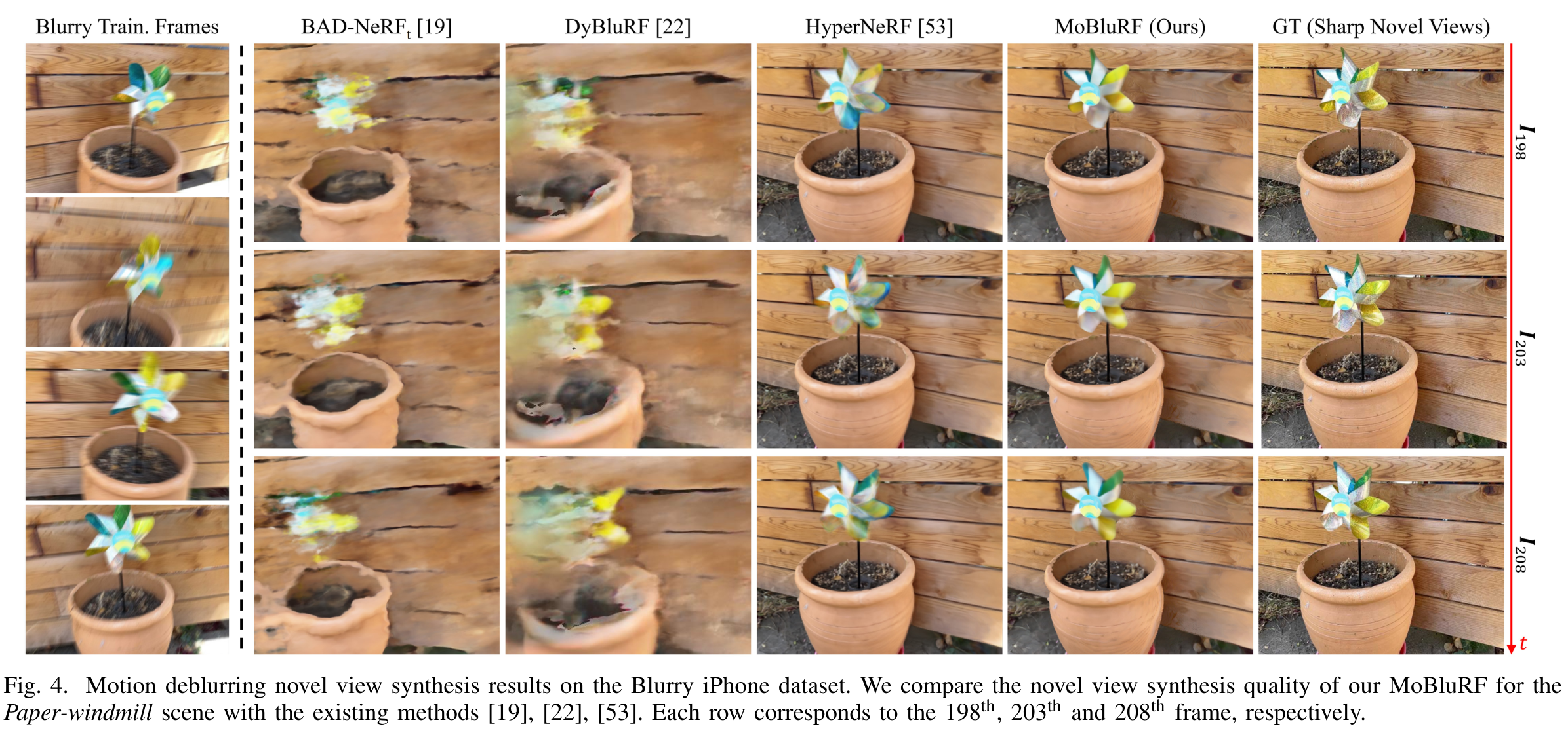
The rotating windmill tests foreground reconstruction alongside a static pot and wooden background. MoBluRF preserves clearer blade boundaries and more coherent surrounding geometry across the three displayed times.
Compared with DyBluRF, average PSNR rises from 25.14 to 25.69, SSIM from 0.891 to 0.893, and LPIPS falls from 0.082 to 0.078. Gains are uneven: Seesaw shows a large PSNR improvement, while Children and Basketball show lower PSNR.
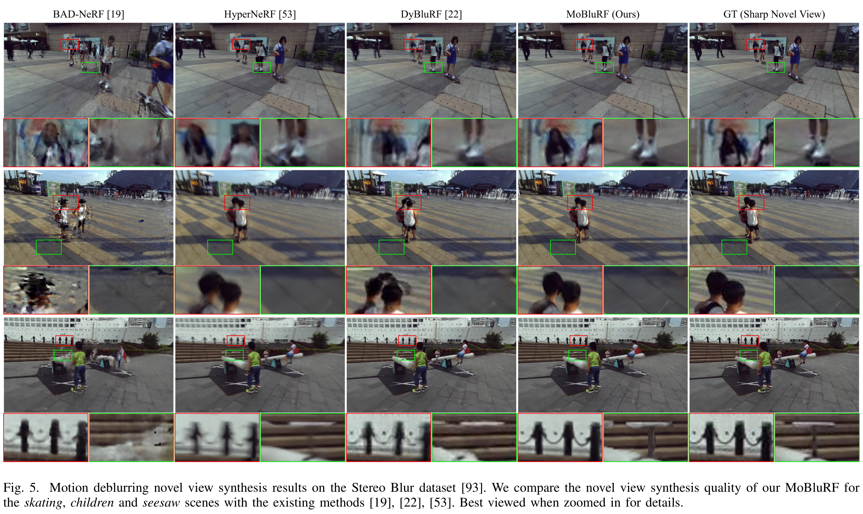
The enlarged person and background regions distinguish foreground deblurring from static reconstruction quality. MoBluRF produces clearer details in several displayed crops, complementing the aggregate metrics without demonstrating superiority on every scene.
The bicycle sequences extend the visual evaluation to naturally blurred video. Helmet and bicycle details appear clearer in MoBluRF’s outputs, but the comparison supplies no sharp reference novel views for quantitative assessment.
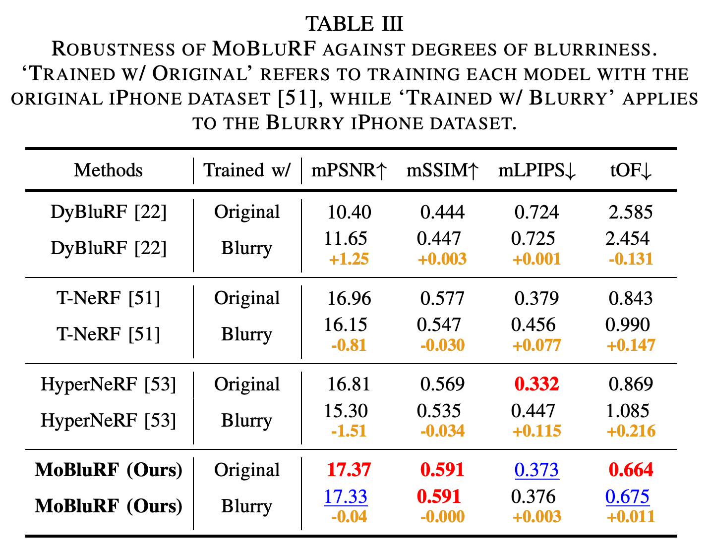
2) Robustness of MoBluRF for Different Degrees of Blurriness: Training on original versus synthesized blurry iPhone videos changes MoBluRF’s average mPSNR from 17.37 to 17.33, mSSIM from 0.591 to 0.591, mLPIPS from 0.373 to 0.376, and tOF from 0.664 to 0.675. T-NeRF and HyperNeRF lose 0.81 and 1.51 mPSNR, respectively, under the same original-versus-blurry comparison.
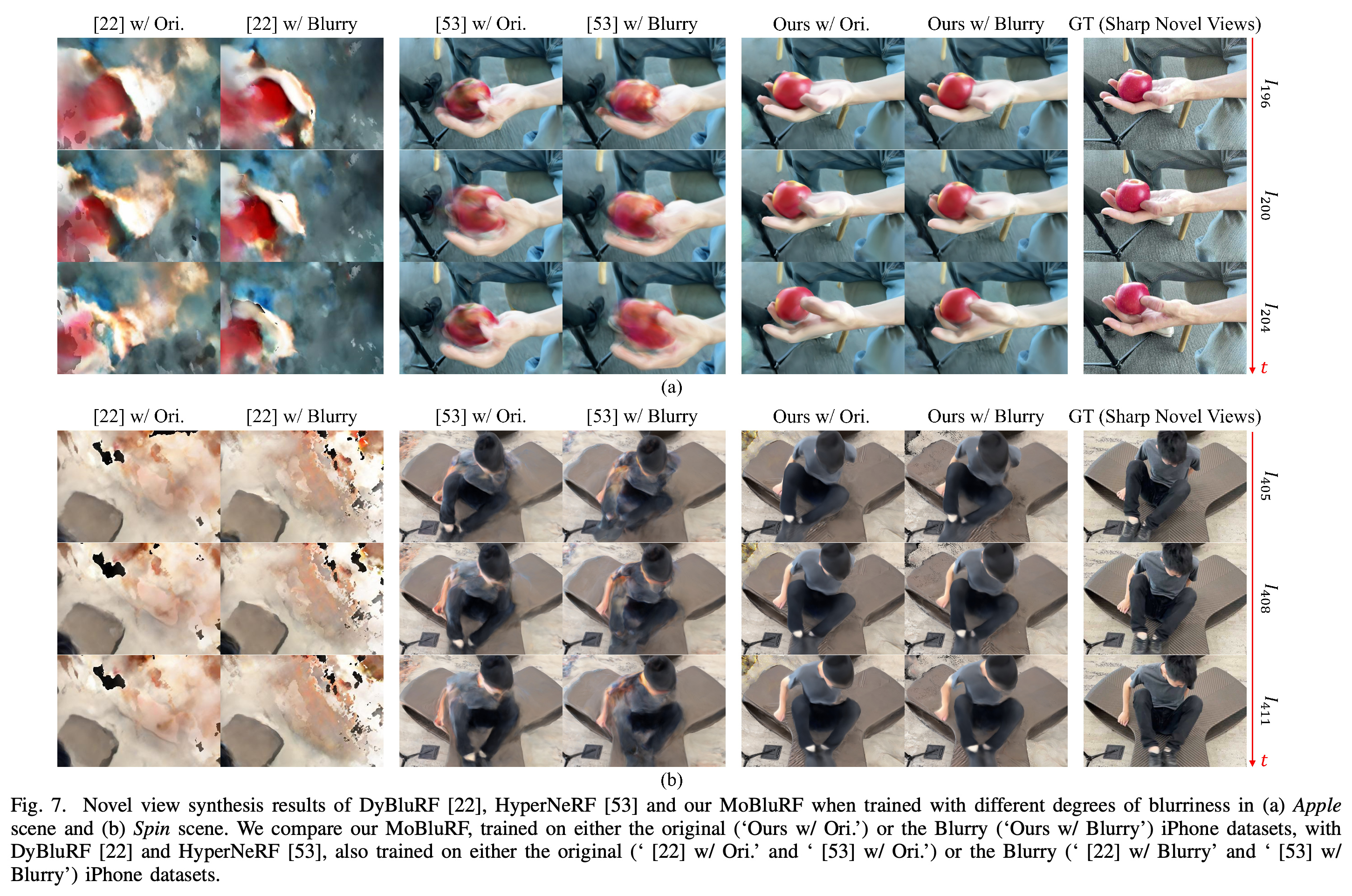
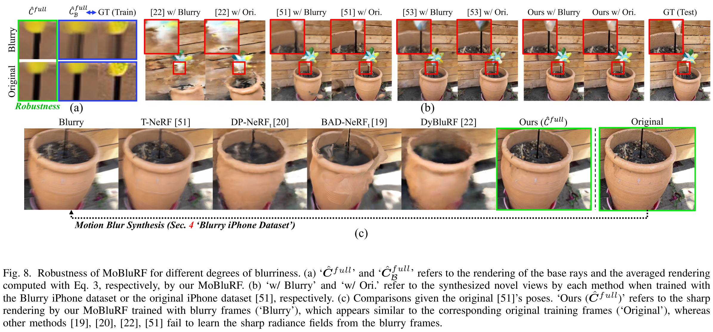
- Figures 7 and 8 show similar sharp reconstructions for MoBluRF across the two training conditions, while the displayed baselines exhibit more blur or misalignment.
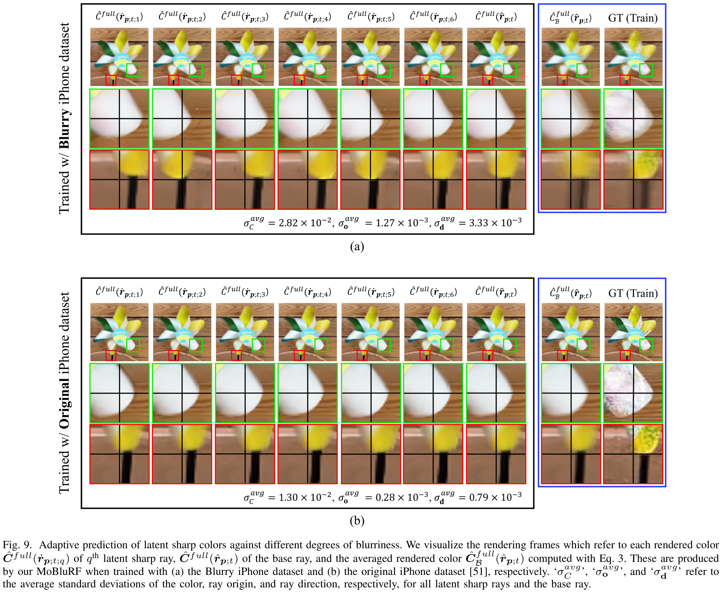
- Figure 9 shows greater variation among predicted latent rays when trained with blurred frames, consistent with the blur model adjusting its contributions to the observations.
- This experiment compares two dataset conditions and does not establish robustness across arbitrary exposure durations or camera blur processes.
MoBluRF’s nearly unchanged results across original and synthesized blurry inputs support robustness within this paired training protocol. HyperNeRF and T-NeRF degrade more, while DyBluRF performs poorly in both conditions.
MoBluRF retains similar object structure under both training conditions in Apple and Spin. HyperNeRF exhibits more blur and DyBluRF more severe reconstruction failures in the selected examples.
The comparison separates the sharp base-ray rendering from the averaged rendering used to explain blurred observations. Their different appearances illustrate how training can reproduce blur while retaining a sharper underlying scene.
Predicted contributions vary more under blurred training than under original training. Average color standard deviation is 2.82 × 10^-2 versus 1.30 × 10^-2, consistent with using more diverse ray contributions to explain blurred observations.
B. Ablation Study on Blurry iPhone dataset
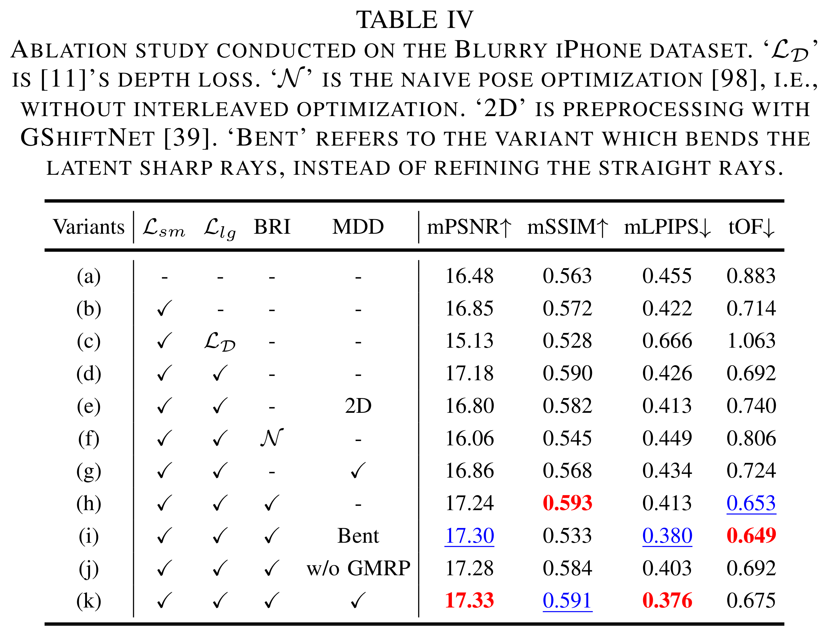
Table IV isolates losses and training stages. Adding the staticness loss changes the baseline’s mPSNR / mSSIM / mLPIPS / tOF from 16.48 / 0.563 / 0.455 / 0.883 to 16.85 / 0.572 / 0.422 / 0.714; adding the proposed geometry loss then reaches 17.18 / 0.590 / 0.426 / 0.692, improving three metrics while slightly worsening perceptual distance.
- Replacing the geometry regularizer with the cited depth loss produces 15.13 / 0.528 / 0.666 / 1.063, supporting the proposed regularizer under this protocol.
- The BRI-only variant reaches 17.24 / 0.593 / 0.413 / 0.653. Adding MDD yields 17.33 / 0.591 / 0.376 / 0.675: perceptual distance improves, while structural similarity and temporal consistency slightly worsen.
- MDD without BRI reaches 16.86 mPSNR and 0.434 mLPIPS; naive pose optimization without interleaving reaches 16.06 mPSNR. Both underperform the full staged procedure.
The full model has the best mPSNR and mLPIPS, while the BRI-only variant has higher mSSIM and lower tOF. Naive pose optimization and MDD without BRI underperform the full staged procedure.
The proposed staticness loss produces cleaner masks than the illustrated flow-derived and squared-log alternatives. The examples support the decomposition mechanism qualitatively; no aggregate segmentation accuracy is reported.
The proposed geometry regularizer preserves a more coherent seated person than the displayed unregularized and conventional-depth-loss variants. Reference depth is unavailable for the novel view, so the figure does not directly measure depth error.
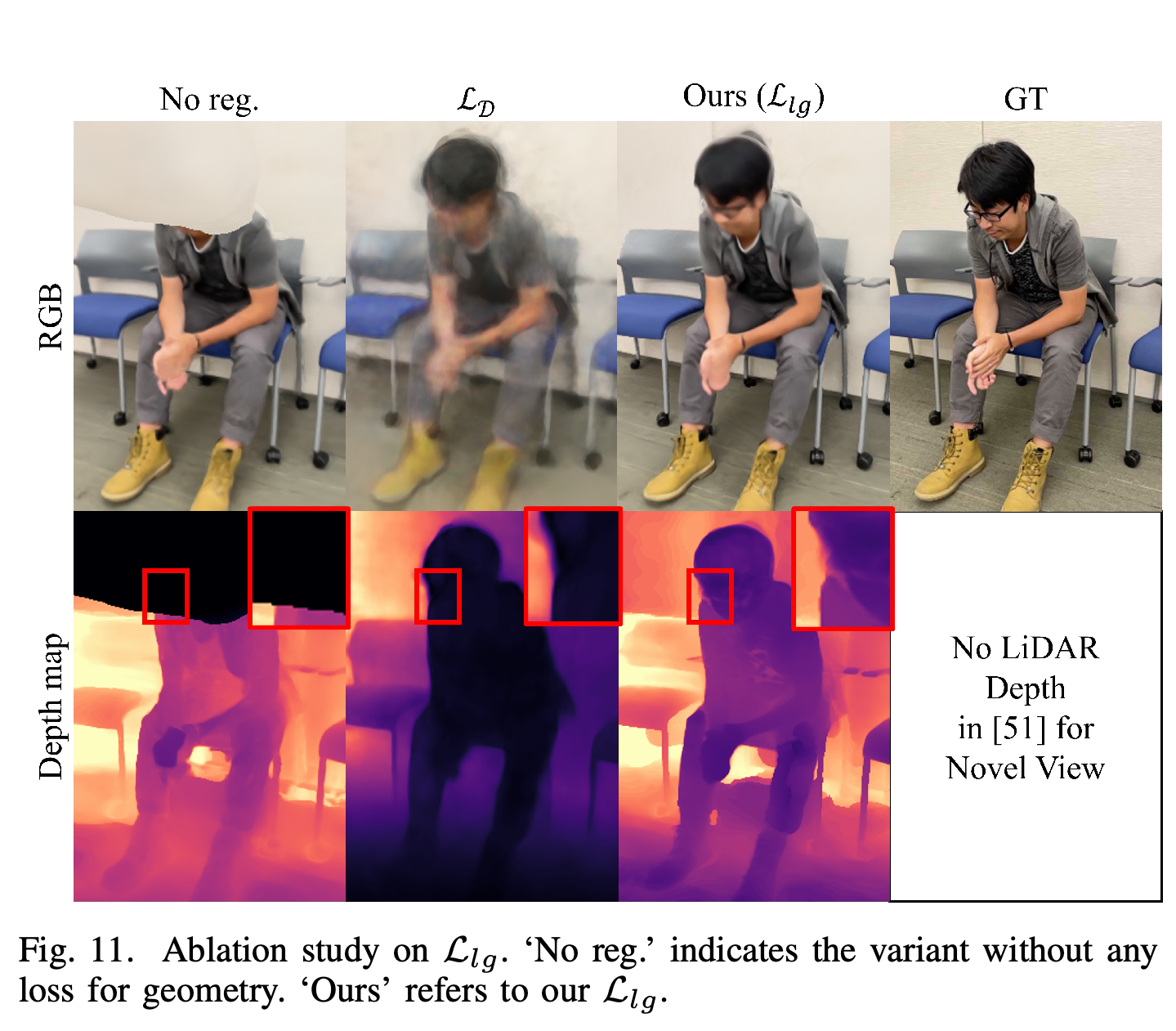
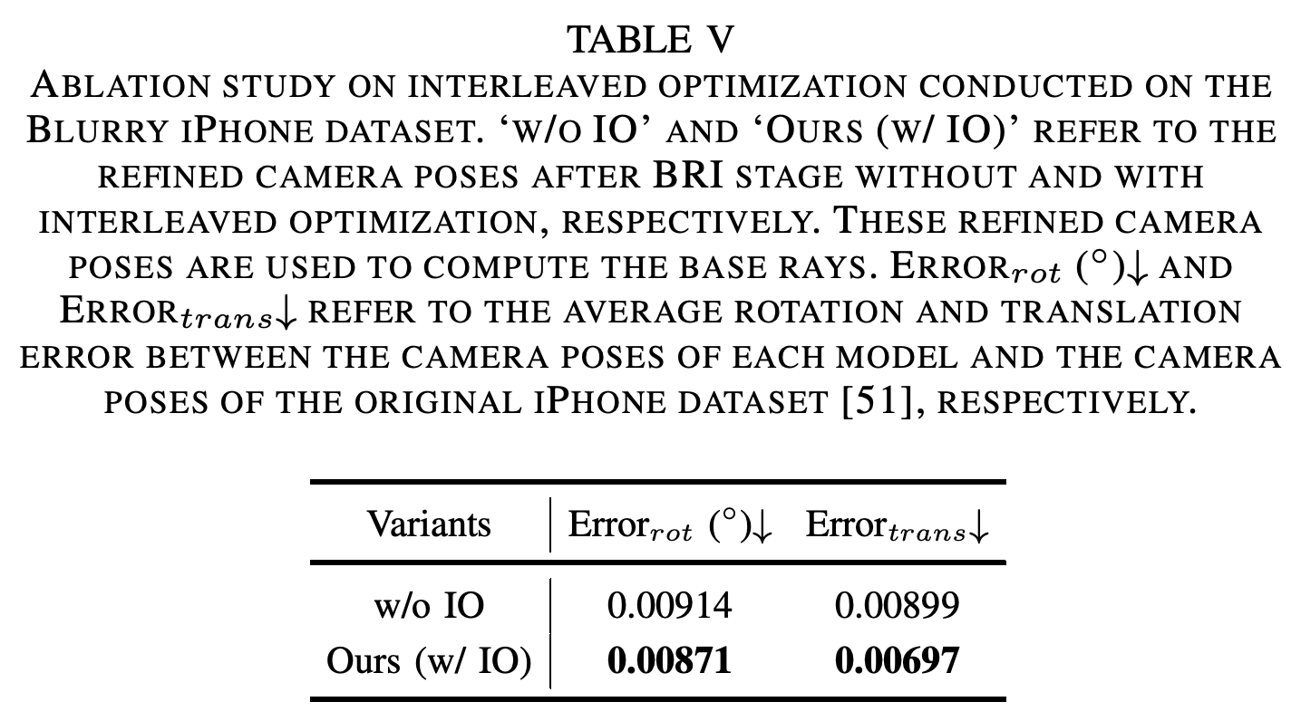
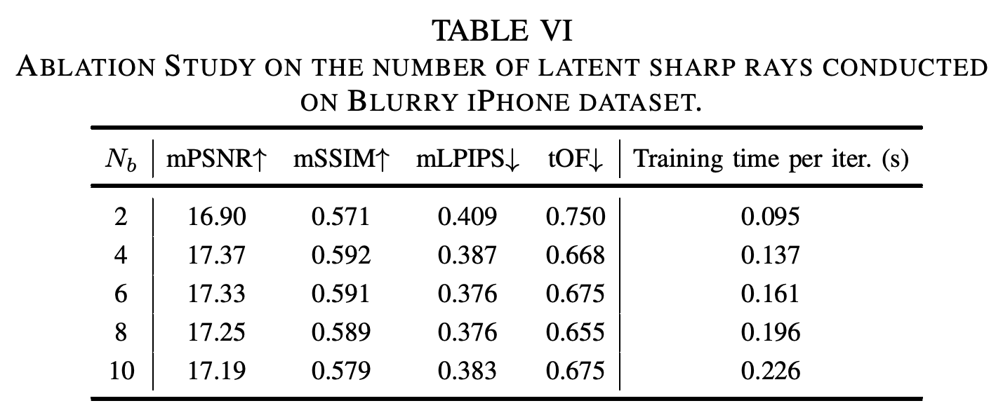
Table V reports lower average pose errors with interleaving: rotation error decreases from 0.00914° to 0.00871°, and translation error from 0.00899 to 0.00697, with no physical translation unit specified. Table VI shows that six latent rays provide a quality–training-cost compromise rather than the best value on every metric.
- At Nb = 2, 4, 6, 8, and 10, training takes 0.095, 0.137, 0.161, 0.196, and 0.226 seconds per iteration on one RTX 3090 Ti with batch size 128.
- Nb = 4 achieves the highest mPSNR, 17.37; Nb = 6 and 8 tie at mLPIPS 0.376; Nb = 8 has the lowest tOF, 0.655.
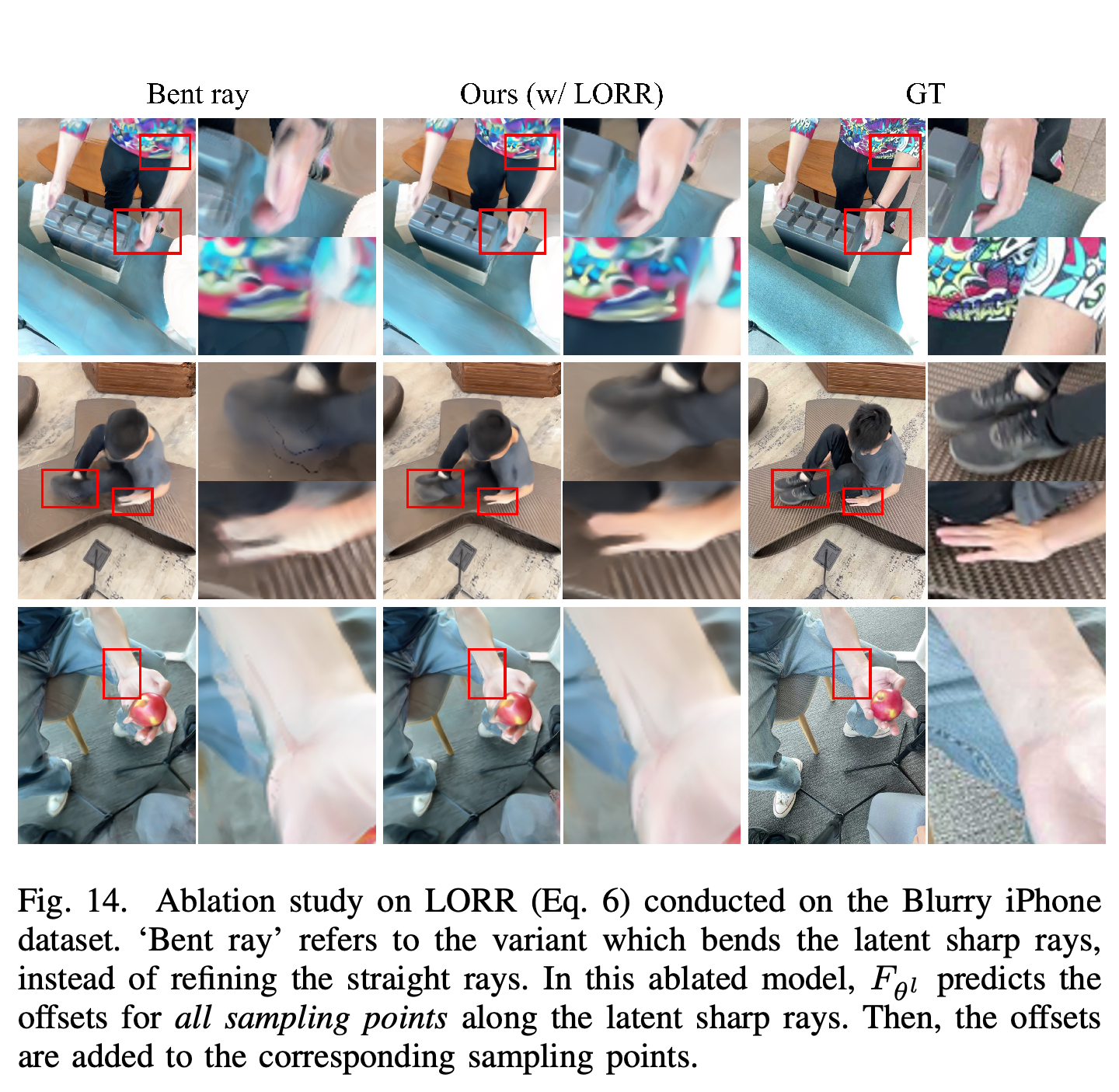
- The bent-ray variant has mSSIM 0.533 versus 0.591 for the full straight-ray refinement model, but better tOF, 0.649 versus 0.675. Removing GMRP worsens mLPIPS from 0.376 to 0.403.
Estimated and original camera trajectories illustrate the pose-refinement effect of interleaved updates. Table V supplies quantitative evidence for the small differences visible in these overlays.
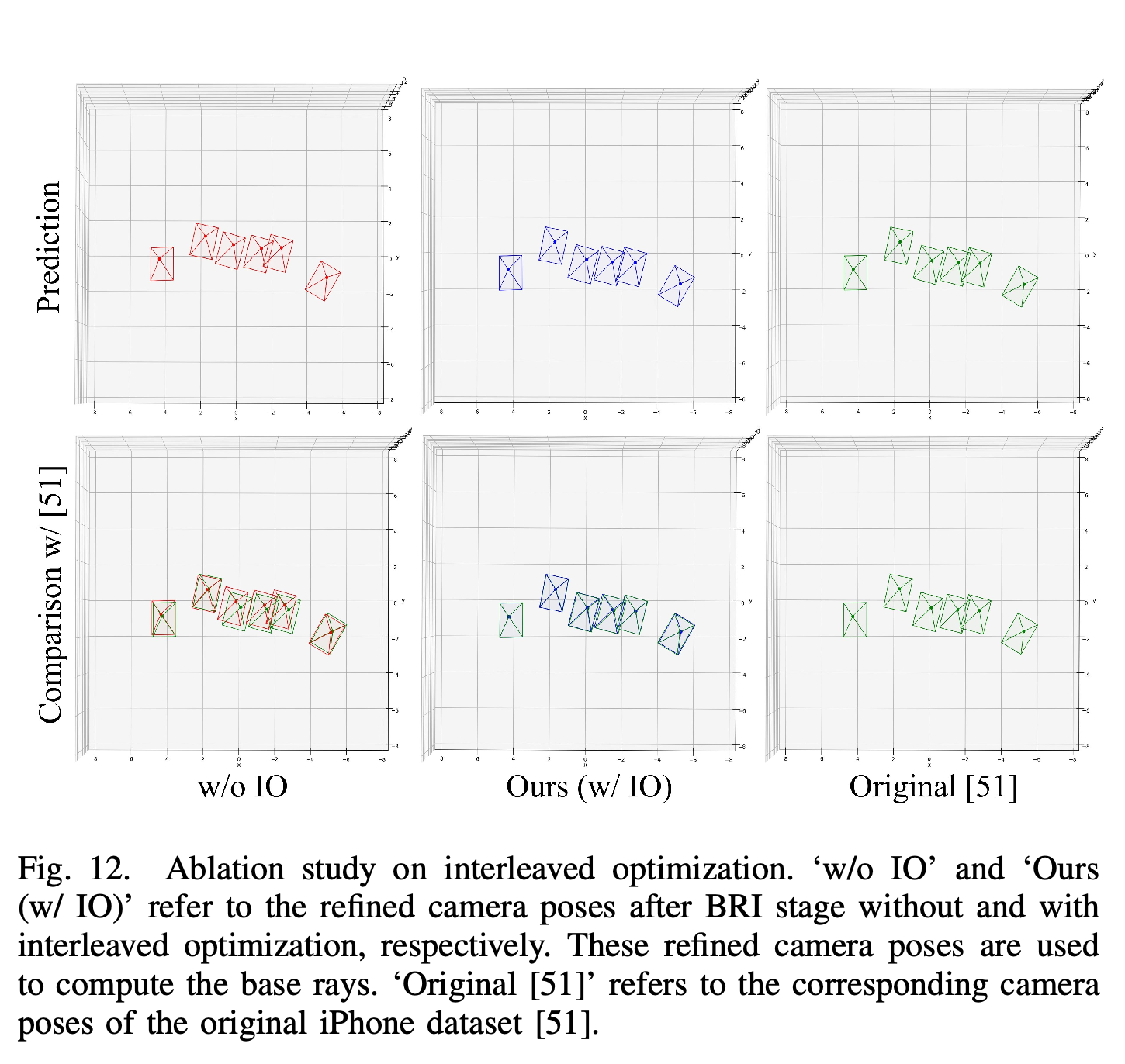
Interleaving lowers rotation error from 0.00914° to 0.00871° and translation error from 0.00899 to 0.00697. No physical translation unit is specified.
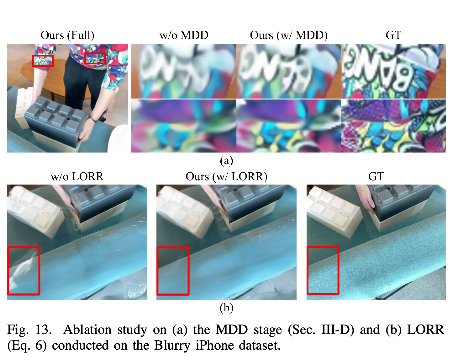
The first comparison shows sharper texture with MDD; the second shows reduced residual object imagery with LORR. These illustrate separate contributions from explicit blur modeling and local motion refinement.
Straight-ray refinement produces cleaner moving-object boundaries than the bent-ray variant in the selected crops. This agrees with the mSSIM difference in Table IV, although the bent-ray variant has better tOF.
Increasing ray count steadily raises training time, but quality is not monotonic. Six and eight rays tie for the lowest mLPIPS, four rays have the highest mPSNR, and eight have the lowest tOF.
C. Ablation Study on Stereo Blur dataset
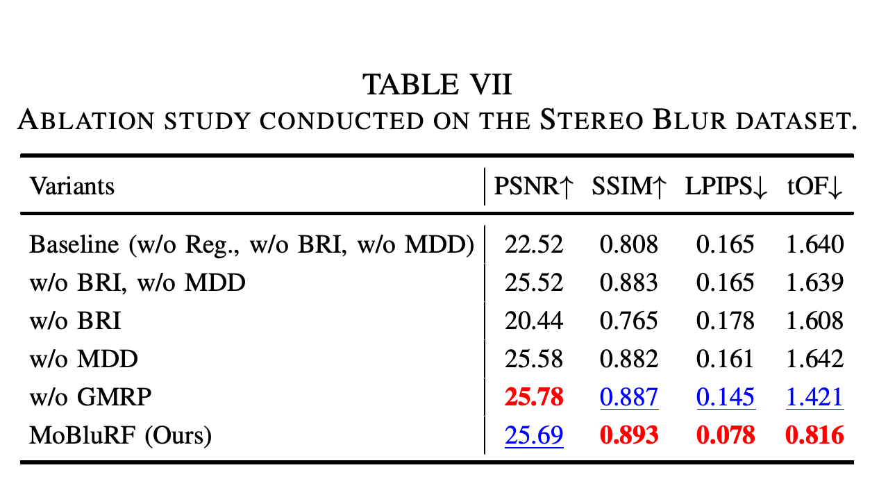
Stereo Blur ablations support the roles of initialization and explicit deblurring. Removing BRI reduces PSNR to 20.44, while removing MDD leaves PSNR at 25.58 but worsens LPIPS to 0.161 and tOF to 1.642, compared with the full model’s 25.69, 0.078, and 0.816.
- Adding the regularizers without either stage improves PSNR from the unregularized baseline’s 22.52 to 25.52, while LPIPS remains 0.165.
- Removing GMRP produces a higher PSNR of 25.78, but lower SSIM of 0.887 and worse LPIPS / tOF of 0.145 / 1.421.
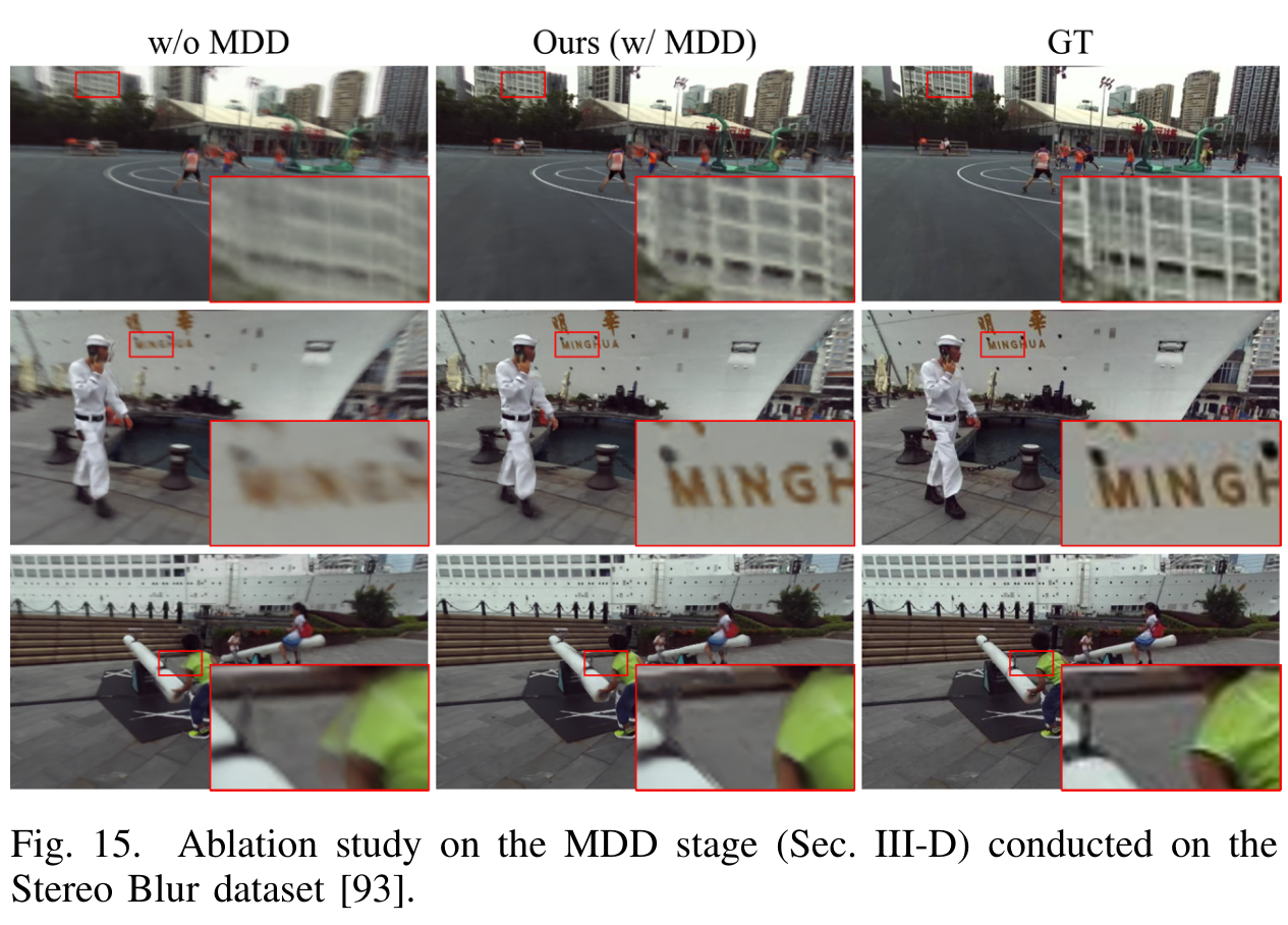
- Figure 15 shows sharper background structure and foreground boundaries with MDD.
The full model reaches LPIPS / tOF of 0.078 / 0.816, compared with 0.161 / 1.642 without MDD. Removing GMRP slightly improves PSNR but substantially worsens perceptual distance and temporal consistency.
The enlarged fence, lettering, and foreground boundary regions appear sharper after MDD. These examples connect the perceptual improvement in Table VII to visible spatial detail.
D. Complexity Comparison
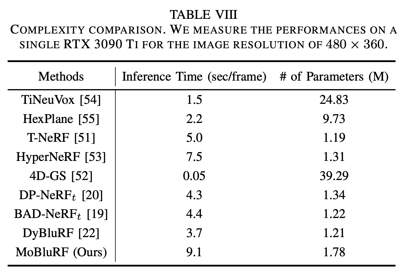
At 480 × 360 resolution on one RTX 3090 Ti, MoBluRF has 1.78 million parameters and takes 9.1 seconds per frame, compared with DyBluRF’s 1.21 million and 3.7 seconds. The listed 4D-GS baseline renders in 0.05 seconds with 39.29 million parameters; MoBluRF has the highest inference time in this comparison.
- The number of latent sharp rays changes training cost but leaves inference unchanged because inference renders a single target ray per pixel.
- The paper prioritizes handling motion blur over rendering speed.
MoBluRF has 1.78 million parameters but the highest listed inference time, 9.1 seconds per frame. The results show that parameter count alone does not describe rendering cost.
E. Limitations and Future Work
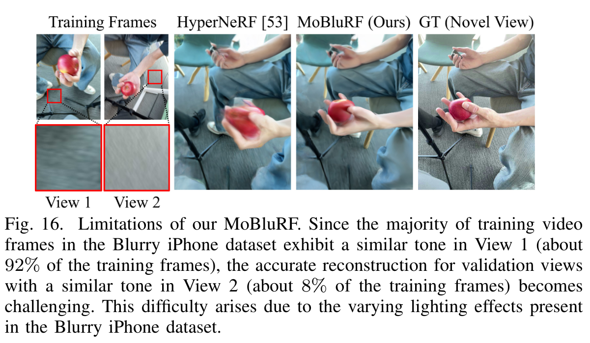
The Blurry iPhone protocol trains from one continuous monocular video per scene and evaluates on two fixed novel-view cameras. View-dependent illumination can therefore be poorly represented: Figure 16 illustrates an approximately 92% versus 8% training-tone imbalance associated with reconstructions that favor the dominant appearance.
- The authors propose reflectance-aware relighting, which models how surfaces respond to illumination, or better-balanced training data as future directions.
- They also propose integrating Gaussian Splatting into the deblurring framework to improve efficiency; this integration is not evaluated in the paper.
- Quantitative evaluation uses synthesized blur, while naturally blurred DAVIS sequences provide qualitative support.
MoBluRF and HyperNeRF favor the dominant training appearance rather than matching the less represented validation tone. The approximately 92% versus 8% imbalance demonstrates an appearance-coverage limitation beyond motion deblurring.
V. Conclusion
The paper concludes that initializing base rays before learning exposure-related ray transformations improves sharp dynamic-scene reconstruction from blurred monocular video. The experiments support combining BRI, MDD, learned static/dynamic decomposition, and geometry regularization, while showing that individual components affect reconstruction, perceptual, and temporal metrics differently.
Appendix
- The supplied 18-page PDF contains no appendix. Its main text is followed by references and author biographies; the attached version is arXiv:2312.13528v3, dated 3 June 2025.
Brief Thoughts
The pose-update schedule is supported by direct ablations: naive pose optimization and deblurring without BRI both underperform the full staged method. The MDD comparisons also show a useful distinction between perceptual sharpness and other objectives, since improved perceptual distance can accompany small losses in structural similarity or temporal consistency. The reported quality gains suit offline reconstruction, while the measured 9.1 seconds per frame constrains interactive use. The Blurry iPhone gains should be read alongside its synthesized blur and pose perturbations. Stereo Blur and qualitative DAVIS examples broaden the evidence, but the PDF reports no uncertainty intervals or repeated-run variability.