Scaling Laws for Looped Mixture of Experts | Summary

Contents

Summary
1 Introduction
2 Related Work
3 Loop Scaling Laws
4 Experiments and Findings
5 Conclusion
Appendix
Brief Thoughts

This article explains the key points of Scaling Laws for Looped Mixture of Experts.

2026-09-30 (arXiv)
Chen, Yanbei, Goyal, Anirudh, Krishnamoorthi, Raghuraman.
Meta AI
Paper

Summary

The paper studies how to allocate language-model capacity between recurrence, repeated passes through shared layers, and Mixture-of-Experts (MoE), which routes each token to a subset of expert networks. At approximately 1.5×10^22 training floating-point operations (FLOPs), its model with 0.3 billion active and 1.3 billion total parameters approximately matches the two-benchmark reasoning average of a non-looped MoE with 0.6 billion active and 2.9 billion total parameters, using 1.5×–1.8× its inference compute at four to five passes. The smaller model still trails on the mean across all 14 benchmarks.
Loop Scaling Laws jointly models active parameters, training tokens, recurrence, and sparsity, the degree to which stored parameters remain inactive for each token. Its effective-parameter mapping, a fitted measure of capacity rather than a count of stored weights, assigns diminishing gains to additional passes and lets greater sparsity raise the saturation limit and extend the approach to it. It predicts held-out loss more accurately than linear, power-law, and sparsity-independent bounded alternatives, which respectively model constant gains, diminishing but unbounded gains, and saturation without a sparsity-dependent recurrence mapping.
The scaling sweep covers 0.3B, 0.6B, and 1.0B active parameters, 100B–500B training tokens, effective expert expansion E∈{1,2,4,8,16}, the ratio of available to selected experts, and recurrence R∈{1,2,3,4,6,8}, the number of passes; B denotes billions. At 5×10^20 training FLOPs, 0.3B MoE models with E≥8 outperform a 1.0B dense model, which uses all its parameters in each pass; at 10^21 FLOPs, recurrence lets smaller MoE models match larger non-looped models on reasoning. Resource-allocation results are predictions from the fitted law, and their memory constraints cover weights alone.

1 Introduction

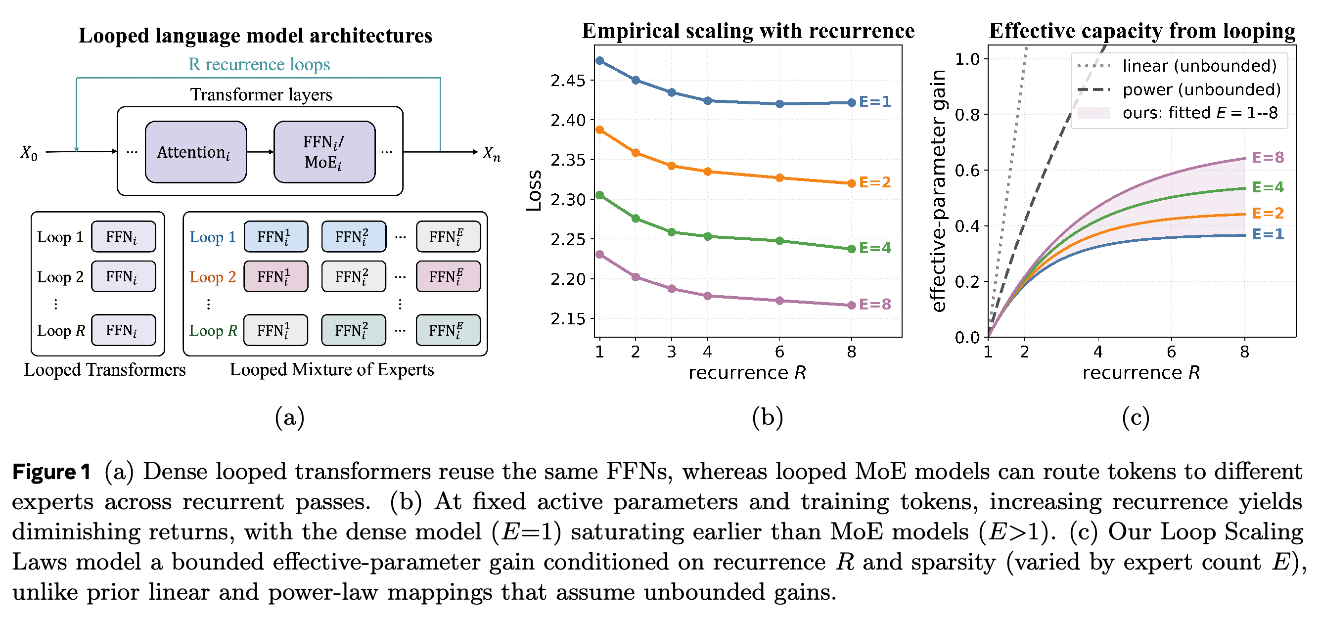
The introduction asks how much effective capacity each recurrent pass adds and whether greater MoE sparsity sustains that gain. At fixed active parameters and training tokens, observed loss falls rapidly over the first few passes and then flattens, with more experts supporting lower loss over more passes. The proposed explanation is that a router, the component selecting experts for each token, can choose different experts across passes even though layer weights are shared.

Looped architectures, empirical recurrence scaling, and bounded effective-capacity gains across expert counts.

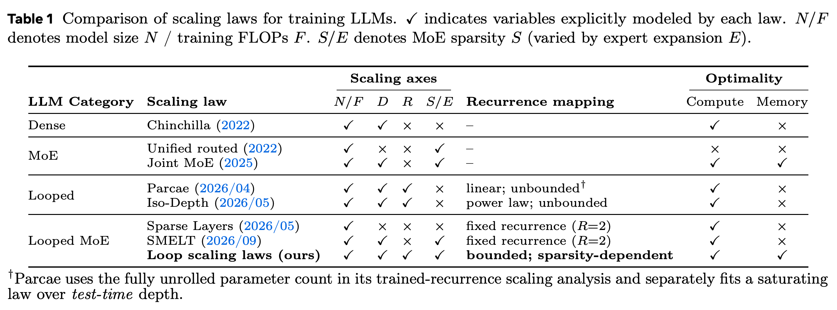
Prior looped-transformer laws represent trained recurrence through linear or power-law capacity mappings, while existing MoE laws model expert expansion without recurrence. Recent looped MoE scaling analyses primarily fix recurrence at R=2. Table 1 identifies the contribution as jointly modeling model size, data, recurrence, and sparsity with a bounded, sparsity-dependent mapping; its footnote distinguishes Parcae, a prior looped-model scaling law, and its linear trained-recurrence analysis from its separately fitted saturating test-time-depth law.

Scaling variables, recurrence mappings, and resource-optimality coverage of prior laws and Loop Scaling Laws.

3 Loop Scaling Laws

The formulation first extends the standard dense language-model scaling law with a recurrence-dependent effective parameter count, then conditions that mapping on MoE sparsity. It separates the capacity attributed to shared-weight computation from the unrolled parameter count, which counts repeated applications of parameters to estimate compute.

3.1 Preliminaries

The baseline is \(\mathcal{L}(N,D)=AN^{\alpha}+BD^{\beta}+c\), where N is model parameters, D is training tokens, A and B are fitted coefficients, α,β<0 are fitted scaling exponents, and c is irreducible loss. Reusing a block with N_loop active parameters for R passes gives N_unroll(R)=N_act+(R−1)N_loop, where N_act counts parameters active in one pass. Under full backpropagation through all passes, training compute is F_train=6N_unroll(R)D and per-token inference compute is F_inf=2N_unroll(R); increasing recurrence leaves stored parameters unchanged.

3.2 Loop Scaling Law

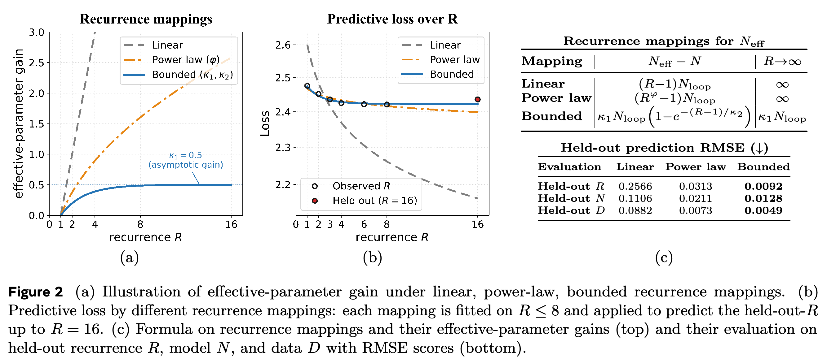
For dense looped models, the proposed mapping is N_eff(R)=N+κ₁N_loop(1−exp(−(R−1)/κ₂)), with κ₁,κ₂>0, and the loss law becomes L(N,D,R)=AN_eff(R)^α+BD^β+c. Here κ₁ sets the asymptotic capacity gain and κ₂ controls its approach; R=1 recovers the non-looped law. When fitted on R≤8 and evaluated at held-out R=16, this bounded form achieves root-mean-square error (RMSE), the square root of mean squared prediction error, of 0.0092 versus 0.0313 for the power-law mapping and 0.2566 for the linear mapping; its infinite-recurrence limit is a property of the fitted function, without an empirical guarantee beyond the observed range.

Dense recurrence mappings and their held-out loss predictions.

3.3 MoE Loop Scaling Law

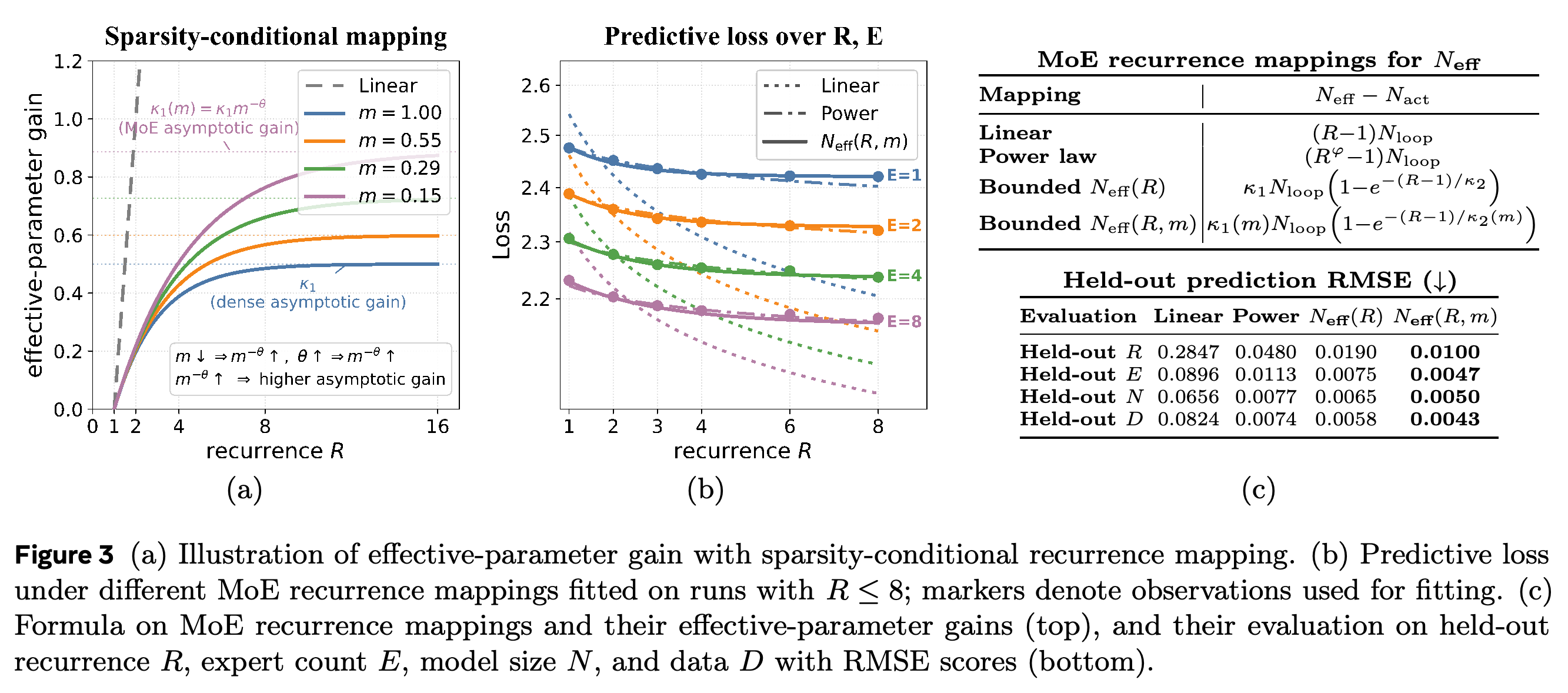
For MoE, m=N_act/N_total∈(0,1] is the active-to-total parameter ratio, so smaller m means greater sparsity. The mapping becomes N_eff(R,m)=N_act+κ₁(m)N_loop(1−exp(−(R−1)/κ₂(m))), with κ_j(m)=κ_jm^(−θ) for j=1,2 and θ≥0; effective expert expansion is E=E_route/k when top-k routing selects k experts from E_route candidates. The outer law is L(N_act,D,R,E,m)=AÊ^δN_eff(R,m)^(α+γ ln Ê)+BÊ^ωD^(β+ζ ln Ê)+c, where Ê is the paper’s monotonic transformation of expert expansion, defined by Ê^(−1)=(E−1+(E_start^(−1)−E_max^(−1))^(−1))^(−1)+E_max^(−1), and δ,γ,ω,ζ,E_start,E_max are fitted coefficients.

For fixed m>0, the gain saturates at κ₁m^(−θ)N_loop; greater sparsity raises this bound and extends the approach over more passes. These limits describe the fitted function and are not empirical guarantees at arbitrary recurrence or sparsity.
The law recovers the dense loop law at E=1 after coefficient reparameterization, the non-looped MoE law at R=1, and the standard dense law when both equal 1.
Held-out RMSE is 0.0100 for recurrence, 0.0047 for expert expansion, 0.0050 for model size, and 0.0043 for data, lower than all three alternative mappings on the same respective splits.

Sparsity-conditioned effective capacity and held-out prediction errors for looped MoE.

4 Experiments and Findings

The experiments assess loss prediction, resource-constrained architecture selection, and downstream benchmark performance. Loss and benchmark comparisons use measured results, while the resource-allocation analyses predict architecture choices from the fitted law.

4.1 Scaling Experiments and Analysis

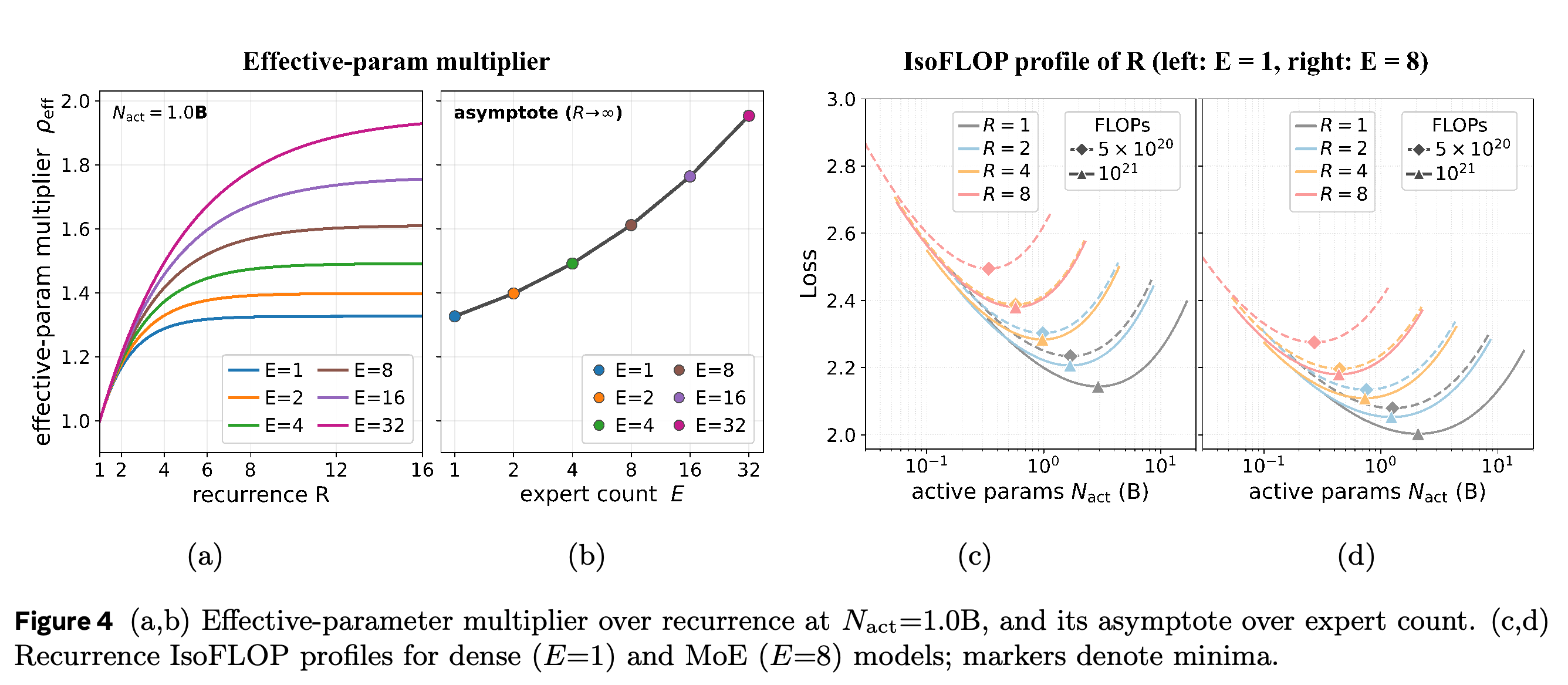
The sweep trains models from scratch over N_act∈{0.3,0.6,1.0}B, D∈{100,200,300,400,500}B, E∈{1,2,4,8,16}, and R∈{1,2,3,4,6,8}. Middle-cycle looping repeats the middle block while leaving the first two and last two layers unshared. The fitted effective-parameter multiplier ρ_eff=N_eff/N_act rises toward a finite, sparsity-dependent asymptote; greater sparsity raises that asymptote and delays saturation.

IsoFLOP comparisons, comparisons at equal training FLOPs, use budgets of 5×10^20 and 10^21. The fitted curves predict lower loss for E=8 than E=1 under the same budget.
At the same active model size, R=2 at 10^21 FLOPs can achieve lower loss than R=1 at 5×10^20 FLOPs. This comparison supports improved quality with additional computation, without establishing that more passes always improve a fixed-budget optimum.

Effective-parameter multipliers and equal-training-compute loss profiles for dense and MoE models.

4.2 Compute- and Memory-Optimal Recurrence and Sparsity

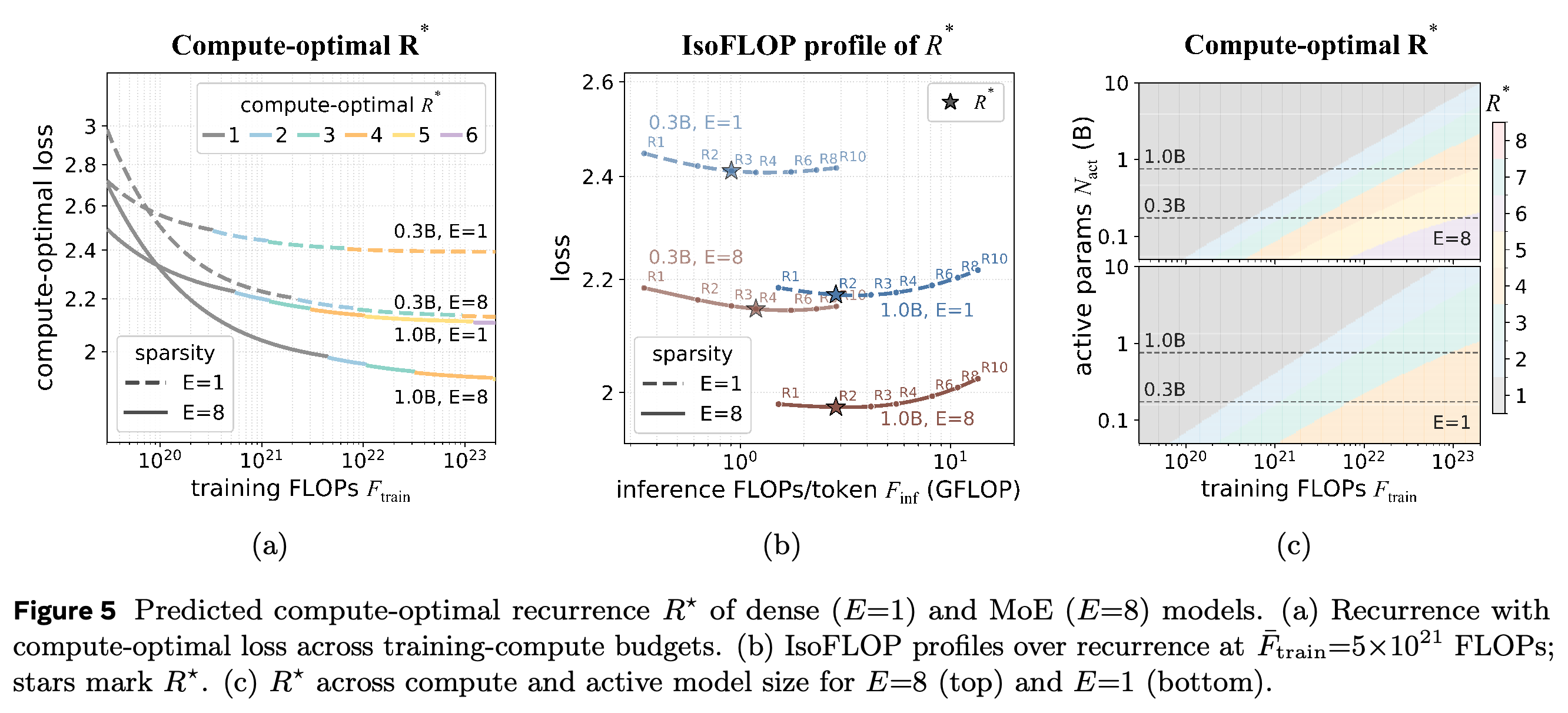
At fixed sparsity and training-compute budget, recurrence selection minimizes predicted loss while requiring the improvement from an additional pass to reach a tolerance ε. The paper sets ε to the fitted-law RMSE, treating smaller predicted improvements as unresolved by the fit, and defaults to R*=1 if no additional pass satisfies the threshold. Predicted optimal recurrence increases with larger training budgets and greater sparsity, and is higher for smaller active models in the evaluated design space.

Predicted compute-optimal recurrence across model sizes, sparsity levels, and training budgets.

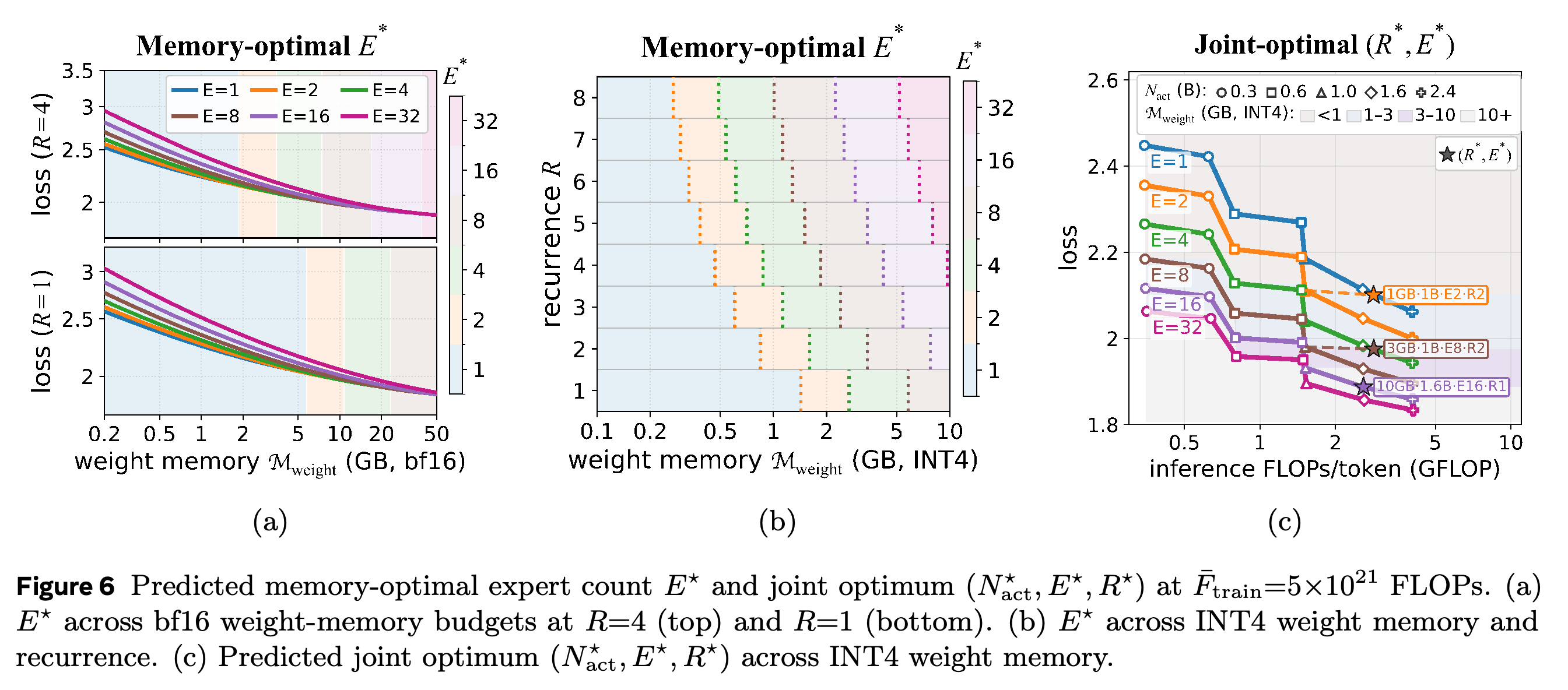
Memory-constrained selection uses M_weight=b_wN_total/8, where b_w is weight precision in bits, and applies the same improvement threshold to expert expansion before jointly searching active model size, expert expansion, and recurrence at matched training compute. At 5×10^21 FLOPs with four-bit integer (INT4) weights, predicted selections include a 1.0B-active model with E=8,R=2 under 3 GB and a 1.6B-active model with E=16,R=1 under 10 GB. Tighter weight memory favors recurrence, while more memory permits greater sparsity; key-value caches, stored attention state, and other runtime memory are outside this optimization.

Predicted memory-optimal expert expansion and joint architecture choices under weight-memory budgets.

4.3 Downstream Scaling with Recurrence and Sparsity

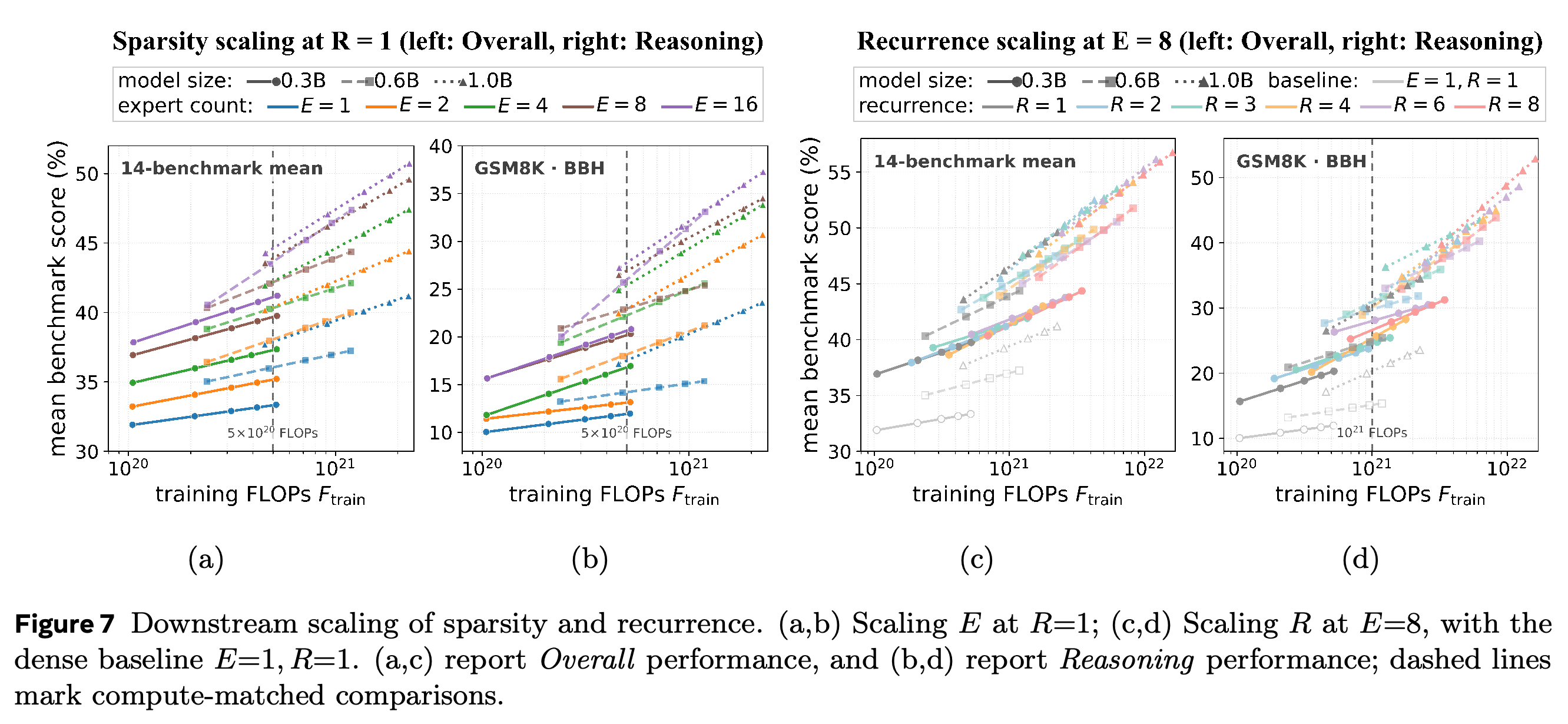
Downstream evaluation reports Overall as the mean across 14 benchmarks and Reasoning as the mean of BIG-Bench Hard (BBH), a reasoning benchmark, and GSM8K, a mathematical word-problem benchmark. At 5×10^20 training FLOPs and R=1, 0.3B MoE models with E≥8 outperform the 1.0B dense model on both aggregates. At 10^21 FLOPs and E=8, the 0.3B model with R≥4 matches or exceeds the 0.6B model with R=1 on Reasoning, while the 0.6B model with R≥3 matches the 1.0B non-looped model.

Downstream Overall and Reasoning performance as expert expansion and recurrence increase.

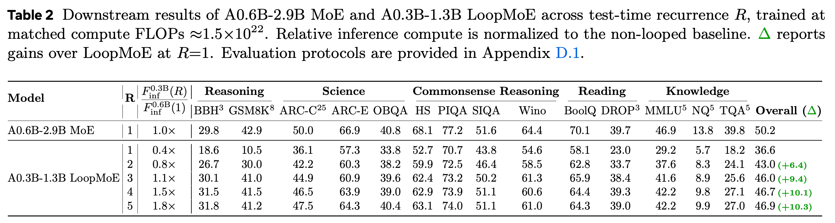
For the trillion-token case study, the law selects R*=5 for A0.3B-1.3B LoopMoE, the looped model with 0.3B active and 1.3B total parameters, which is trained for approximately 3T tokens against approximately 6T tokens for A0.6B-2.9B MoE at approximately 1.5×10^22 training FLOPs; T denotes trillions. At test-time R=5, LoopMoE scores 31.8 on BBH and 41.2 on GSM8K versus 29.8 and 42.9 for the larger model, but Overall is 46.9 versus 50.2 and relative inference compute is 1.8×. Varying the same LoopMoE checkpoint from R=1 to R=5 raises Overall from 36.6 to 46.9, a 10.3-point gain.

At R=4, the smaller model uses 1.5× baseline inference compute and scores 31.5 on BBH, 41.5 on GSM8K, and 46.7 Overall.
The reasoning-match claim describes approximately comparable performance across the two reasoning benchmarks. The smaller model scores higher on BBH and lower on GSM8K at R=4–5, and remains below the larger model on Overall.

Compute-matched trillion-token results for A0.6B-2.9B MoE and A0.3B-1.3B LoopMoE across test-time recurrence.

5 Conclusion

The conclusion argues for choosing recurrence and sparsity together according to compute and weight-memory constraints. The experiments support improved held-out loss prediction in the tested setting and a tradeoff between stored parameters and inference computation on reasoning tasks. Alternative looping strategies, broader model scales, recurrent-state optimization, and early-exit gating, stopping computation before all passes when appropriate, remain future work.

Appendix

A Reduced Forms of Loop Scaling laws: A.1 Dense Loop Scaling Law proves that R=1 gives N_eff=N and recovers the standard dense loss law. A.2 MoE Loop Scaling Law derives the reductions at E=1, R=1, and their intersection, including the coefficient reparameterization required by the transformed expert variable.
B Expert-Path Diversity Across Recurrence measures the number of distinct experts selected across passes, averaged over tokens and recurrent layers and normalized by the number selected per pass. On the same validation set of 800 prompts, diversity at R=8 rises from 1.5088±0.0529 for E=2 to 1.7035±0.0861 for E=8, reported as mean ± standard deviation, while dense models remain at 1. This routing statistic supports the proposed motivation but does not establish that expert diversity causes the fitted capacity gains.
C Scaling Experiments and Parametric Fitting: C.1 Training Details specifies the same open-licensed, web-heavy mixture supplemented with math, code, knowledge, and science data, a 2,048-token context, and a llama tokenizer with a 202k vocabulary. Training uses AdamW, an adaptive optimizer, with β₁=0.9, β₂=0.95, ε=10^−15, weight decay 0.1, and gradient clipping at 1.0, on 64 NVIDIA H100 96 GB graphics processing units. The scaling sweep applies next-token prediction loss only to the final pass; the trillion-token LoopMoE adds supervision at every pass to support variable recurrence at inference.
C.2 Model Ladder and Scaling Sweep defines five active model scales, {0.3,0.6,1.0,1.6,2.4}B, while the measured scaling sweep uses the first three. The joint architecture search evaluates 300 configurations over those five scales, E∈{1,2,4,8,16,32}, and R∈{1,…,10}; 1.6B and 2.4B active models, E>16, and R>8 therefore involve extrapolation. Fitted parameter counts exclude embeddings, the input-output token representations, whereas the reported active and total counts in the model ladder include them.
C.3 Parametric Fitting first fits the R=1 subset, then jointly estimates coefficients across all scaling axes; comparisons hold out R=16, E=16 for MoE, model size 1.0B, or D∈(400,500]B and fit on the remaining observations for each split. The final law uses more than 1,000 loss observations, initializes with scipy.optimize.curve_fit using nonlinear least squares and a mean squared error objective, and refines with scipy.optimize.minimize using L-BFGS-B, a numerical optimization method, and a log-Huber objective, a robust fitting loss. Fitted recurrence coefficients are κ₁=0.3682, κ₂=1.4037, θ=0.3286, with full-data RMSE 0.0037; allowing separate sparsity exponents for κ₁ and κ₂ leaves RMSE at 0.0037, supporting the shared-exponent choice for these observations.
C.4 Bootstrap Results of the MoE Loop Scaling Law assesses fit sensitivity by refitting 100 subsets, each containing 90% of observations sampled without replacement. The reported 90% percentile intervals, bounded by the 5th and 95th percentiles of the refits, are [0.3658,0.3723] for κ₁, [1.3896,1.4243] for κ₂, and [0.3183,0.3350] for θ. At 5×10^21 training FLOPs, the reported architecture intervals collapse to the selected configurations at 1 GB, 3 GB, and 10 GB, indicating stability under this resampling procedure.
D Downstream Scaling and Evaluation: D.1 Downstream Evaluation Protocols uses the Language Model Evaluation Harness, an evaluation framework, at https://github.com/EleutherAI/lm-evaluation-harness with vLLM, the inference backend, at https://github.com/vllm-project/vllm, bfloat16 precision, a 16-bit floating-point format, and greedy decoding, selecting the highest-scoring next token, for generation tasks. The 14 benchmarks span reasoning, science, commonsense, reading, and knowledge, with task-specific metrics and numbers of demonstration examples. BBH uses 3 examples, GSM8K 8, ARC-Challenge, a science question-answering benchmark, 25, DROP, a reading benchmark requiring discrete reasoning, 3, and MMLU, a multitask knowledge benchmark, Natural Questions, a question-answering benchmark, and TriviaQA, a trivia question-answering benchmark, 5 each; the remaining tasks use 0.
D.2 Compute-Matched Trillion-Token Experiment details Algorithm D.1: for each candidate recurrence, compute N_unroll(R), set D_target^R=F̄_train/[6N_unroll(R)] for training budget F̄_train, predict loss, and select recurrence using the RMSE-based improvement threshold. This procedure selects R*=5 for the smaller LoopMoE. Test-time evaluation varies R∈{1,2,…,5} and normalizes its inference FLOPs to the larger non-looped reference.

Brief Thoughts

The held-out comparisons support explicitly modeling the interaction between recurrence and sparsity: the sparsity-conditioned mapping improves predictions across all four tested axes, including against a bounded mapping without sparsity conditioning. Expert-path measurements offer a plausible explanation for this interaction, but remain observational.

The demonstrated deployment tradeoff is fewer stored parameters in exchange for more inference computation on reasoning tasks. Table 2’s 46.9 versus 50.2 Overall scores and 1.8× inference-compute ratio constrain broader efficiency claims, while the architecture search excludes runtime memory and relies partly on extrapolation. Stable refits quantify sensitivity to the available observations; they do not establish transfer to other data mixtures, looping strategies, hardware latency, or much larger models.