The GAN is dead; long live the GAN! A Modern GAN Baseline | Summary

This article explains the key points of The GAN is dead; long live the GAN! A Modern GAN Baseline.

• 2025-01-09 (arXiv), 38th Conference on Neural Information Processing Systems (NeurIPS 2024)
• Huang, Yiwen, Gokaslan, Aaron, Kuleshov, Volodymyr, Tompkin, James.
• Brown University, Cornell University
• Paper
• Github

Read this article in Korean

Summary

• Generative adversarial networks (GANs), which train an image generator against a discriminator that scores real and generated images, can suffer unstable training and limited sample diversity. At comparable network capacity, R3GAN achieves a Fréchet Inception Distance (FID), an image-distribution comparison metric where lower is better, of 2.75 versus StyleGAN2’s 3.78 on unconditional FFHQ-256 generation, producing 256 × 256 face images without class labels.
• The method combines relativistic pairing GAN (RpGAN), which compares discriminator scores for generated and real samples, with R₁ and R₂, penalties on discriminator input gradients for real and generated data respectively. Under stated assumptions and sufficiently small learning rates, the objective supports local convergence, meaning convergence when training starts sufficiently near equilibrium, and enables a simpler architecture built from residual blocks that add learned transformations to identity connections.
• R3GAN recovers all 1000 StackedMNIST modes, distinct combinations of stacked handwritten digits, and achieves FID 1.96 on the CIFAR-10 small-image benchmark and 2.09 on ImageNet-64, a 64 × 64 version of the ImageNet image dataset, with one network evaluation per generated image. The paper establishes a competitive baseline in these settings; global convergence, higher-resolution ImageNet scaling, and large-scale generation from text descriptions remain unverified.

1 Introduction

The paper connects unstable adversarial objectives with GAN architectures that accumulate specialized mechanisms to compensate. It stabilizes the objective, removes nonessential StyleGAN2 features, and then modernizes the generator and discriminator while keeping capacity roughly comparable. The PDF title is “The GAN is dead; long live the GAN! A Modern Baseline GAN,” and its code URL is https://www.github.com/brownvc/R3GAN.

2 Serving Two Masters: Stability and Diversity with RpGAN + R₁ + R₂

Stable training can still produce a generator that omits parts of the data distribution. The authors combine the diversity-oriented RpGAN objective with zero-centered gradient penalties, which encourage discriminator input gradients toward zero, to address stability and diversity together.

2.1 Traditional GAN

The traditional objective is L(θ,ψ) = E_z[f(Dψ(Gθ(z)))] + E_x[f(−Dψ(x))], where θ and ψ parameterize the generator and discriminator, z is sampled noise, x is real data, and E denotes expectation. The generator Gθ minimizes L, the discriminator Dψ maximizes it, and the paper uses f(t) = −log(1 + e^(−t)). Although direct optimization over distributions has favorable properties, practical parameter updates move generated samples relative to discriminator decision boundaries and can produce mode dropping, the omission of subsets of the training distribution, or non-convergence.

2.2 Relativistic f-GAN

RpGAN replaces independent real and generated scores with L(θ,ψ) = E_z,x[f(Dψ(Gθ(z)) − Dψ(x))], judging each generated sample relative to a real sample. The paper cites prior loss-landscape results, concerning how the objective varies over candidate solutions, that exclude mode-dropping local minima under their assumptions. Such a landscape does not guarantee that gradient-based training reaches an optimum.

2.3 Training Dynamics of RpGAN

The authors demonstrate that unregularized RpGAN need not converge and extend prior convergence analysis to RpGAN with either R₁ or R₂. These penalties are R₁ = (γ/2)E_real[‖∇xDψ(x)‖²] and R₂ = (γ/2)E_generated[‖∇xDψ(x)‖²], where ∇x denotes differentiation with respect to the input and γ controls regularization strength. The local result requires a generator capable of matching the real distribution, a discriminator constant near the real-data support, regularity and sensitivity conditions near equilibrium, and sufficiently small learning rates; it does not guarantee convergence from arbitrary initialization.

2.4 A Practical Demonstration

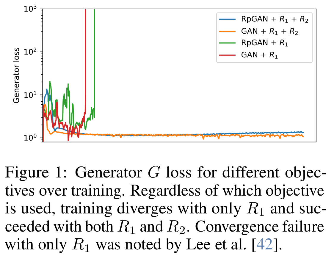
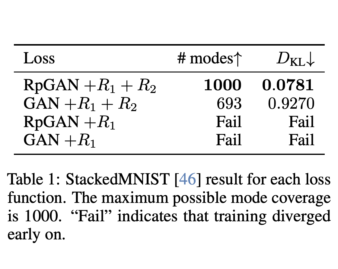
A small residual network without normalization, which standardizes intermediate activations, is tested on StackedMNIST using a pretrained digit classifier to measure coverage and reverse Kullback–Leibler (KL) divergence, the discrepancy between generated mode frequencies and the uniform target distribution. Figure 1 shows early divergence with R₁ alone for both objectives, whereas adding R₂ stabilizes both; Table 1 then distinguishes diversity, with RpGAN recovering 1000 modes and divergence 0.0781 versus 693 modes and 0.9270 for the traditional objective. Varying γ from 0.1 to 100 did not stabilize the R₁-only case, supporting penalties on both distributions in this experiment.

Both R₁-only runs diverge early, whereas adding R₂ keeps the displayed generator-loss trajectories bounded for both objectives. This supports regularizing generated and real data in this experiment; diversity requires a separate measurement.

With both penalties, RpGAN covers 1000 modes with reverse KL divergence 0.0781, while the traditional objective covers 693 with 0.9270. Stable training alone therefore does not ensure full mode recovery.

3 A Roadmap to a New Baseline — R3GAN

The roadmap compares configurations A–E on FFHQ at 256 × 256, training each until the discriminator sees 5 M real images and keeping capacity roughly comparable. It removes style mapping and injection, which transform and insert latent controls; weight modulation/demodulation, which adjusts convolution weights using those controls; noise injection; mixing and path-length regularization, which constrain style combinations and sensitivity to latent changes; latent normalization; minibatch standard deviation, which supplies a batch-diversity statistic; equalized learning rate, which rescales weights during computation; and lazy regularization, which applies penalties intermittently.

• The stripped baseline reduces latent dimension to 64 and learning rate from 2.5 × 10⁻³ to 5 × 10⁻⁵. Retained choices include the Adam optimizer with its first-moment momentum coefficient β₁ = 0, no activation normalization, bilinear resampling to change image resolution, and leaky ReLU, an activation with a nonzero slope for negative inputs.
• The modernized architecture uses separate resolution-transition layers and two residual blocks per resolution. Each block uses 1 × 1, 3 × 3, and 1 × 1 convolutions, with no bias in the final convolution; fix-up initialization zeroes that final layer and scales the other two initializations by L⁻⁰·²⁵, where L counts residual blocks, to control activation variance without normalization.
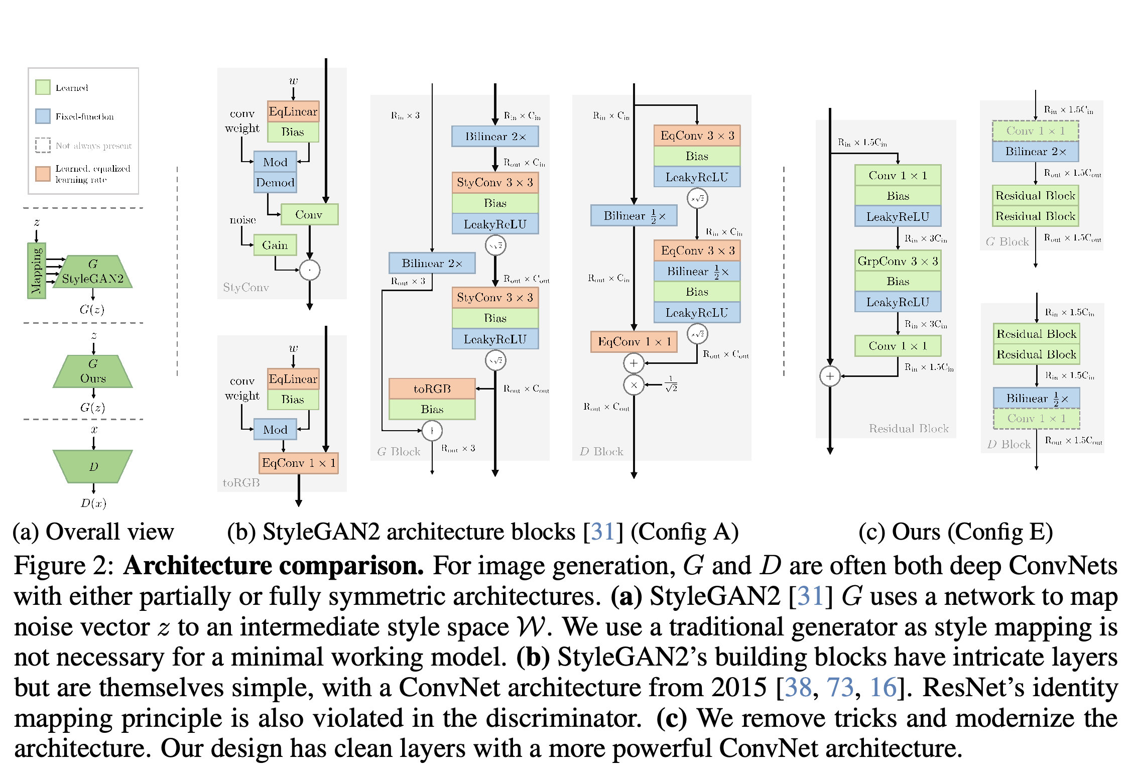
• The final design uses 3 × 3 grouped convolution, which processes channels in groups, with group size 16. An inverted bottleneck swaps the wider and narrower channel dimensions to increase grouped-convolution capacity without increasing model size; Figure 2 contrasts this design with StyleGAN2.

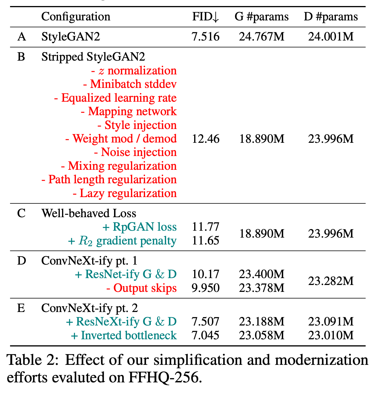
Removing StyleGAN2 features worsens FID from 7.516 to 12.46. The regularized loss improves it to 11.65, and successive architecture changes reduce it to 7.045 after the same 5 M-real-image training exposure; the comparison does not isolate architecture improvements under alternative objectives.

The final model removes the intermediate style-mapping pathway and separates resampling from residual processing. Its simpler blocks retain a symmetric generator/discriminator organization while changing the convolutional architecture.

4 Experiments Details

The experiments separate the short architectural roadmap from final models trained to convergence with optimized hyperparameters and schedules. Evaluation covers unconditional face and StackedMNIST generation, plus class-conditional CIFAR-10 and downsampled ImageNet generation, where class labels guide sampling. Measures include FID, mode coverage, recall as a measure of sample diversity, and number of function evaluations (NFE), the network evaluations required to generate a sample.

4.1 Roadmap Insights on FFHQ-256 [29]

Table 2 reports FID 7.516 for StyleGAN2, 12.46 after stripping its features, 11.77 after introducing RpGAN, and 11.65 after adding R₂. Residual modernization reaches 9.950 after removing output skips, connections that combine generator outputs across resolutions; grouped convolutions reach 7.507, and the inverted bottleneck reaches 7.045. Architecture changes account for most of the recovery from the stripped baseline in this short-run comparison, although the experiment does not establish that their gains require the new objective.

4.2 Mode Recovery — StackedMNIST [53]

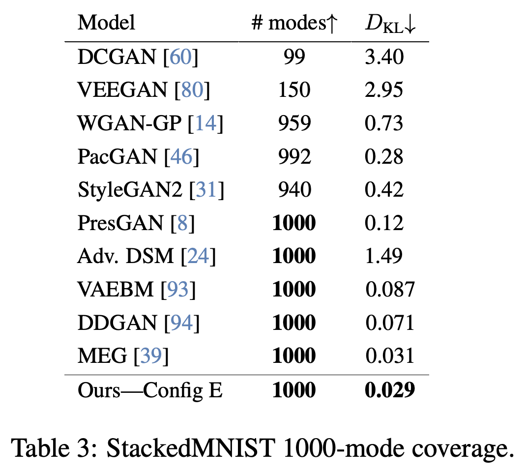
With the final architecture, R3GAN recovers all 1000 StackedMNIST modes and reaches KL divergence 0.029. Table 3 reports 940 modes and 0.42 for StyleGAN2; several methods also recover every mode but have higher divergence, including DDGAN, a denoising diffusion GAN, at 0.071 and MEG, a maximum-entropy generator, at 0.031. Full coverage and closeness to uniform mode frequencies are distinct outcomes.

Several methods reach all 1000 modes, but R3GAN has the lowest listed KL divergence at 0.029. This distinguishes recovering every mode from reproducing uniform mode frequencies.

4.3 FID — FFHQ-256 [29] (Optimized)

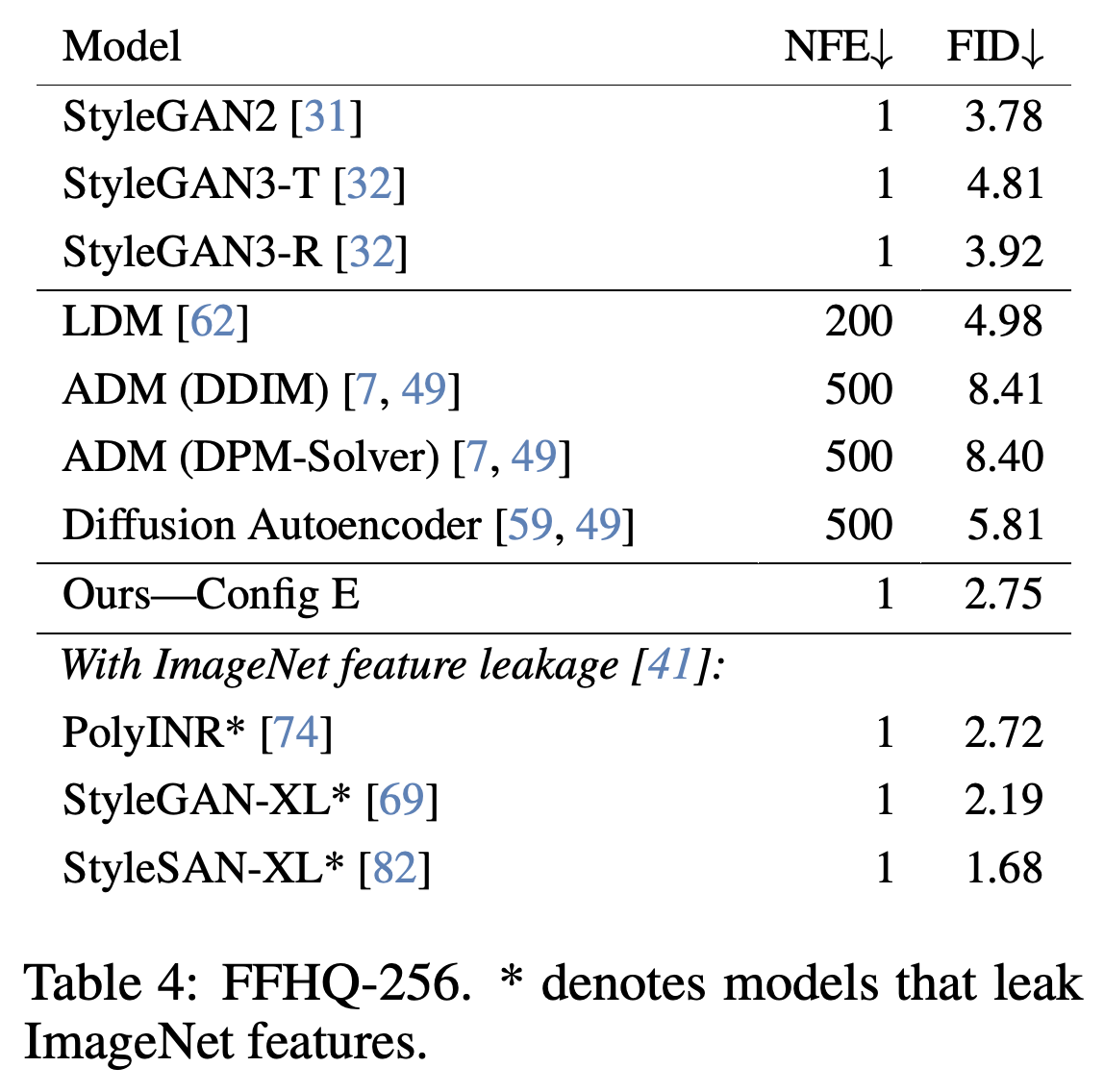
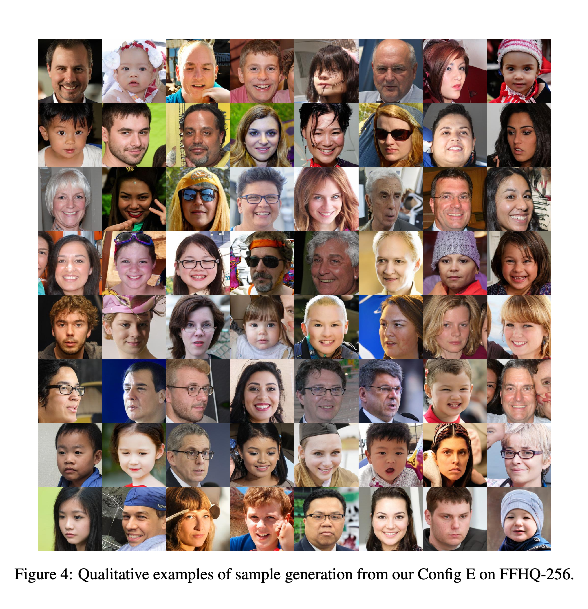
After optimized training to convergence, unconditional FFHQ-256 generation reaches FID 2.75 at NFE 1, compared with StyleGAN2 at 3.78 and the listed diffusion-based methods, which generate through repeated denoising, at 4.98–8.41 with 200–500 evaluations. Table 4 separately identifies models using pretrained ImageNet features that can influence FID evaluation; some score lower, including StyleSAN-XL at 1.68. Figure 4 supplies qualitative face samples, and R3GAN omits the additional consistency regularization discussed in this section, a constraint encouraging consistent discriminator behavior under image transformations.

R3GAN improves on the listed StyleGAN2/3 and diffusion results while using one evaluation. The separately marked ImageNet-feature models include lower FID values, qualifying the comparison.

4.4 FID — FFHQ-64 [33]

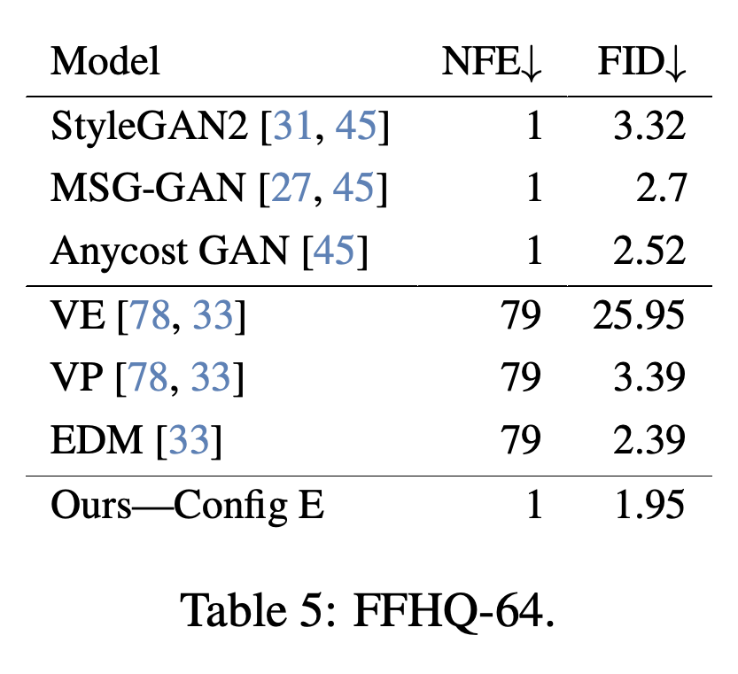
For FFHQ-64, the authors remove the two highest-resolution stages from the FFHQ-256 architecture. Table 5 reports FID 1.95 with one evaluation versus 2.39 with 79 evaluations for EDM, the diffusion baseline from “Elucidating the Design Space of Diffusion-Based Generative Models.” The resulting generator has fewer than half as many parameters as EDM.

R3GAN reaches FID 1.95 with one evaluation, compared with EDM at 2.39 with 79. These figures compare distributional error and evaluation counts; they do not directly measure hardware latency.

4.5 FID — CIFAR-10 [37]

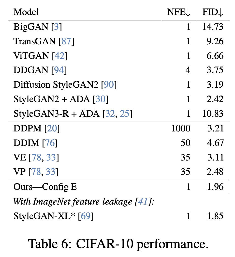
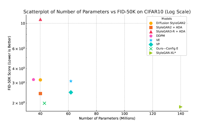
On class-conditional CIFAR-10, R3GAN reaches FID 1.96 with one evaluation, compared with StyleGAN2 + ADA, adaptive discriminator augmentation, at 2.42 and the listed diffusion baselines at 2.48–4.67. Figure 3 compares FID with parameter counts; Table 9 specifies 20.78 M generator and 21.28 M discriminator parameters. StyleGAN-XL scores 1.85, but the paper separates its use of pretrained ImageNet discriminator features because FID also relies on an ImageNet-trained feature extractor.

R3GAN’s 1.96 FID is below the listed baselines outside the separately marked ImageNet-feature row. StyleGAN-XL reaches 1.85 under that different feature-pretraining condition.

R3GAN combines low FID with substantially fewer total parameters than StyleGAN-XL. Parameter count compares capacity, but does not establish training cost or per-evaluation speed.

4.6 FID — ImageNet-32 [6]

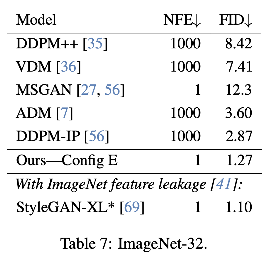
For class-conditional ImageNet-32, the model is widened to approximately match StyleGAN-XL’s 84 M-parameter generator; Table 9 gives R3GAN’s generator size as 82.91 M. R3GAN achieves FID 1.27 with one evaluation, versus 2.87 with 1000 evaluations for DDPM-IP, a denoising diffusion model trained with input perturbation, and 1.10 for StyleGAN-XL in the separately marked ImageNet-feature comparison. The authors report a 60% smaller discriminator than StyleGAN-XL and no pretrained ImageNet classifier.

R3GAN achieves FID 1.27 with one evaluation, below the listed diffusion results at their reported sampling settings. StyleGAN-XL’s separately marked 1.10 remains lower.

4.7 FID — ImageNet-64 [6]

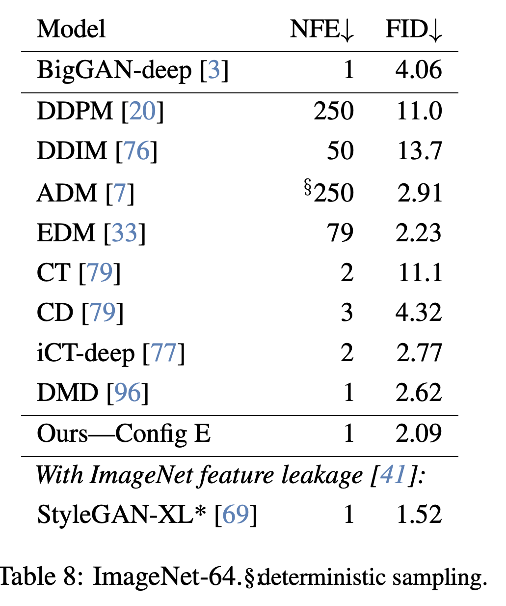
Adding one resolution stage produces an ImageNet-64 generator with 103.57 M parameters, approximately 104 M in the main text, compared with about 300 M for the cited diffusion backbones. Table 8 reports FID 2.09 at one evaluation, versus EDM’s 2.23 at 79 evaluations and DMD, a model trained through distribution matching distillation for one-step generation, at 2.62 with one evaluation. StyleGAN-XL achieves 1.52 in the separately marked ImageNet-feature comparison.

R3GAN’s 2.09 FID is below EDM’s 2.23 and DMD’s 2.62, including a one-evaluation comparison with DMD. The separately marked StyleGAN-XL result is 1.52, and ADM’s evaluation count carries a deterministic-sampling qualification.

4.8 Recall

Recall reaches a peak of 0.57 on CIFAR-10 versus 0.47 for StyleGAN-XL. R3GAN obtains 0.53 on FFHQ-64 and 0.49 on FFHQ-256, compared with StyleGAN2’s 0.43 on FFHQ-256. ImageNet-32 recall is 0.63, comparable to ADM, the diffusion baseline from “Diffusion Models Beat GANs on Image Synthesis,” while ImageNet-64 recall is 0.59 versus approximately 0.63 for many diffusion models and 0.48 for BigGAN-deep; lower FID therefore does not imply higher diversity in every comparison.

5 Discussion and Limitations

The authors prioritize a minimal generation baseline and remove features useful for image editing, inversion, which maps images back to latent inputs, and controllable synthesis. They omit latent-conditioned adaptive normalization, which adjusts normalization using the latent input, and attention, which combines information across spatial locations; higher-resolution ImageNet and large-scale text-to-image scaling remain unverified. They also acknowledge potential misuse through fabricated images of people, while Appendix D documents multi-day or multi-week training costs.

The face grid shows variation in appearance, pose, expression, and background at 256 × 256 resolution. It accompanies the quantitative results without providing a controlled human comparison or an independent coverage estimate.

6 Conclusion

The conclusion presents R3GAN as a simplified GAN baseline whose regularized relativistic objective supports local convergence under the stated conditions and permits modern architecture design. The reported experiments show competitive performance within its parameter-size class on the evaluated datasets.

Appendix

The appendices provide convergence analysis, implementation details, unsuccessful design choices, sample grids, and training traces.

• A Local convergence analyzes training as a dynamical system using eigenvalues of its update Jacobian, the matrix describing local changes in the update.
• B DiracRpGAN: A demonstration of non-convergence studies a point-mass generator and linear discriminator: θ(t)² + ψ(t)² remains constant along unregularized continuous-time trajectories, preventing non-equilibrium trajectories from approaching equilibrium, while a positive gradient penalty yields local convergence for sufficiently small learning rates.
• C General Convergence Results adapts the analysis of Mescheder et al. C.1 Assumptions requires a generator capable of matching the real distribution, a discriminator constant near the real-data support, f′(0) ≠ 0 and f″(0) < 0, and regular equilibrium manifolds, sets of equivalent parameterizations, with sufficient discriminator sensitivity to distributional deviations. C.2 Convergence proves at least linear local convergence to these sets for either R₁ or R₂ at sufficiently small learning rates and states that the result extends to both penalties together.
• D Hyperparameters, training configurations, and compute describes implementation on the official StyleGAN3 code base, reusing generator exponential moving average (EMA), a smoothed history of generator weights, augmentation, and evaluation support. Table 9 lists training durations of 10, 250, 200, 100, 1000, and 1000 Mimg, meaning millions of images, for StackedMNIST, CIFAR-10, FFHQ-256, FFHQ-64, ImageNet-32, and ImageNet-64 respectively. Cosine burn-in schedules, smooth initial transitions to target settings, adjust learning rate, penalty strength, Adam’s second-moment averaging coefficient β₂, EMA half-life, and augmentation probability; mixed precision, computation using multiple numerical formats, uses BFloat16 after 16-bit floating-point FP16 impaired training.
• E Negative Results and Future Work reports worse FID with the smooth activation alternatives GELU, Gaussian error linear units, Swish, and SMU, smoothing maximum units; group normalization, which standardizes groups of feature channels, brought no improvement, and Pixel-Shuffle/Unshuffle, which rearranges channels and spatial positions, produced artifacts without low-pass filtering. More capacity at low resolutions generally accelerated overfitting, Adam β₂ = 0.999 caused ImageNet stability problems, and applying R₁ and R₂ only once every 8 minibatches caused convergence failure on StackedMNIST and several toy datasets. Attention and transformer architectures, which use attention-based processing, were not experimentally evaluated.
• F Qualitative Results provides generated examples for Stacked-MNIST, FFHQ-256, FFHQ-64, CIFAR-10, ImageNet-32, and ImageNet-64 in Figures 5–10. These grids illustrate generated samples but do not independently establish distribution coverage or comparative perceptual quality.
• G Training Curves presents discriminator and generator losses, R₁ and R₂ measurements, and FID over wall time for CIFAR-10, FFHQ-64, FFHQ-256, ImageNet-32, and ImageNet-64 in Figures 11–15. The displayed runs show declining FID but do not measure variability across independent runs.
• The NeurIPS Paper Checklist states that error bars were omitted because repeated training runs were too expensive and that code was unavailable at submission time despite the abstract’s URL. Appendix D reports 7 hours for StackedMNIST and 4 days for CIFAR-10 on 8 × NVIDIA L40, and roughly 3 weeks for FFHQ on 8 × NVIDIA A6000. Its ImageNet compute prose combines “one day on 32 H100s” with “about 5000 H100 hours,” which are not arithmetically equivalent; Table 9 separately lists 32 GPUs for ImageNet-32 and 64 for ImageNet-64.

  Brief Thoughts

The clearest evidence separates training stability, diversity, and architectural capacity: Figure 1 and Table 1 distinguish stable training from mode coverage, while Table 2 attributes most short-run FID recovery to architecture changes. The theorem establishes local behavior under explicit assumptions; reliability from initialization rests on the reported experiments. Missing run-to-run uncertainty, substantial training costs, and untested higher-resolution settings limit the reach of the benchmark comparisons.