목차

• 1. Learning Structured Output Representation using Deep Conditional Generative Models
  • 1.1. Introduction
  • 1.2. Related Work
  • 1.3. Preliminary: Variational Auto-Encoder
  • 1.4. Deep Conditional Generative Models for Structured output Prediction
    • 1.4.1. Output Inference and Estimation of the Conditional Likelihood
    • 1.4.2. Learning to predict structured output
    • 1.4.3. CVAE for Image Segmentation and Labelling
      • 1.4.3.1. Training with multi-scale prediction objective
      • 1.4.3.2. Training with Input Omission Noise
  • 1.5. Experiments
  • 1.6. Conclusion
• 2. Tensorflow로 확인
• Reference

본 글에서는 Variational AutoEncoder를 개선한 Conditional Variational AutoEncoder (이하 CVAE)에 대해 설명하도록 할 것이다. 먼저 논문을 리뷰하면서 이론적인 배경에 대해 탐구하고, Tensorflow 코드(이번 글에서는 정확히 구현하지는 않았다.)로 살펴보는 시간을 갖도록 하겠다. VAE에 대해 알고 싶다면 이 글을 참조하길 바란다.

1. Learning Structured Output Representation using Deep Conditional Generative Models

1.1. Introduction

구조화된 Output 예측에서, 모델이 확률적인 추론을 하고 다양한 예측을 수행하는 것은 매우 중요하다. 왜냐하면 우리는 단지 분류 문제에서처럼 many-to-one 함수를 모델링하는 것이 아니라 하나의 Input에서 많은 가능한 Output을 연결짓는 모델이 필요하기 때문이다. CNN이 이러한 문제에 효과적인 모습을 보여주었지만, 사실 CNN은 복수의 mode를 갖는 분포를 모델링하기에는 적합하지 않다.

이 문제를 다루기 위해서는 Output Representation Learning과 구조화된 예측을 위한 새로운 Deep Conditional Generative Model이 필요하다. 즉, 고차원의 Output Space를 Input 관측값에 조건화되어 있는 생성 모델로 모델링해야하는 것이다. 변분 추론과 Directed Graphical Model의 최근 발전에 기반하여 본 논문은 CVAE를 새로운 모델로서 제안한다. 이 모델은 Directed Graphical Model로서 Input 관측값이 Output을 생성하는 Gaussian 잠재 변수에 대한 Prior를 조절한다. 모델은 조건부 Log Likelihood를 최대화하도록 학습하게 되며, 우리는 이 과정을 SGVB: Stochastic Gradient Variational Bayes의 프레임워크 안에서 설명할 것이다. SGVB에 대해 미리 알고 싶다면 이 글을 참조하도록 하라. 또한 더욱 Robust한 예측 모델을 만들기 위해 우리는 Input Noise Injection이나 Multi-scale Prediction Training Method 등을 소개할 것이다.

실험에서 본 모델의 효과성을 보이도록 할 것인데, 특히 데이터가 일부만 주어졌을 때 구조화된 Output을 모델링하는 데에 있어 확률적 뉴런의 중요성을 보여줄 것이다. 데이터셋은 Caltech-UCSD Birds 200과 LFW를 사용하였다.

1.2. Related Work

(중략)

1.3. Preliminary: Variational Auto-Encoder

이 Chapter 역시 대부분 생략하도록 하겠다. 자세한 설명은 글 서두에 있는 링크를 클릭하여 살펴보도록 하자. 최종적으로 VAE의 목적함수만 정리하고 넘어가겠다.

1.4. Deep Conditional Generative Models for Structured output Prediction

변수에는 3가지 종류가 있다. Input 변수 x, Output 변수 y, 잠재 변수 z가 바로 그것이다. $\mathbf{x}$ 가 주어졌을 때, $\mathbf{z}$ 는 아래와 같은 사전 확률로 부터 추출된다.

그리고 output $\mathbf{y}$ 는 아래 분포로 부터 생성된다.

baseline CNN과 비교하여 잠재 변수 $\mathbf{z}$ 는 Input이 주어졌을 때 Output 변수에 대한 조건부 분포에서 복수의 mode를 모델링하는 것을 허용하기 때문에 제안된 CGM (조건부 생성 모델) 을 one-to-many mapping 모델링에 적합하게 만든다. 위 식에 따르면 잠재 변수의 사전 확률은 Input 변수에 의해 조절되는 것처럼 보이지만, 이러한 제한은 잠재 변수를 Input 변수에 독립적으로 만들어 해소할 수 있다.

Deep CGM은 조건부 Conditional Log Likelihood를 최대화하면서 학습된다. 이 목적 함수는 종종 intractable 하기 때무에 우리는 SGVB 프레임워크를 적용할 것이다. ELBO는 아래와 같다.

물론 위 식의 우변의 두 번째 항은 Monte-Carlo Estimation을 통해 경험적으로 값을 얻을 수 있다. 이 기법에 대해 알고 싶다면 이 글을 참조하라. 다시 포현하면 아래와 같다.

$L$ 은 Sample의 개수이며 이 때,

본 논문은 이 모델을 CVAE라고 부를 것이다. 이 모델은 복수의 MLP로 구성되는 데 크게 3가지의 요소를 갖고 있다.

1) Recognition Network

2) Prior Network

3) Generation Network

이 네트워크 구조를 디자인할 때, baseline CNN 위에 CVAE의 구성요소를 올릴 것이다. 아래 그림에서 (d)를 확인해보자.

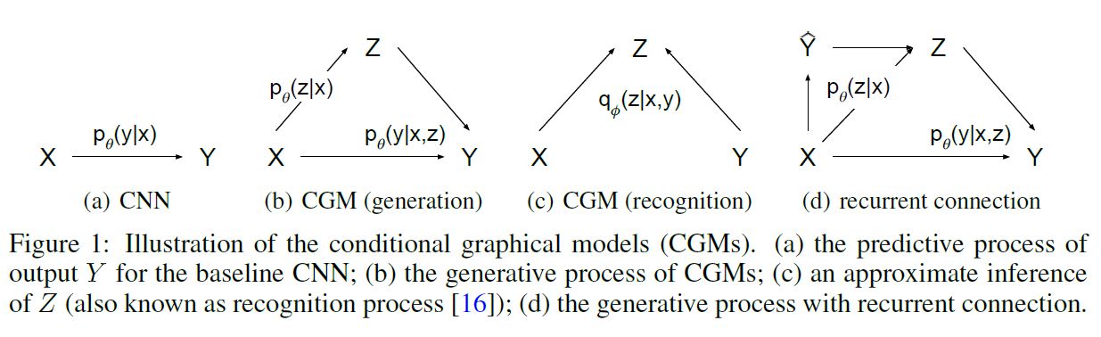
직접적인 Input $\mathbf{x}$ 뿐만 아니라 CNN으로부터 만들어진 최초의 예측 값 $\hat{\mathbf{y}}$ 는 Prior Network로 투입된다. 이러한 순환 연결은 구조화된 Output 예측 문제에서 효과적으로 합성곱 네트워크를 깊게 만들면서 이전의 추측을 수정하여 예측값을 연속적으로 업데이트하는 과정에 적용된 바 있다. 우리는 또한 이러한 순환 연결이, 설사 단 한 번의 반복에 그치더라도, 굉장한 성능 향상을 이끌어낸다는 사실을 발견했다. 네트워크 구조에 대한 자세한 사항은 이후에 설명할 것이다.

1.4.1. Output Inference and Estimation of the Conditional Likelihood

모델 파라미터가 학습되면 CGM의 생성 과정을 따라 Input으로부터 Output에 대한 예측을 수행하게 된다. 모델을 평가하기 위해서 우리는 $\mathbf{z}$ 에 대한 Sampling 없이 Deterministic Inference를 수행할 수 있다.

또는 사전 확률로부터 복수의 $\mathbf{z}$ 를 추출한 뒤 사후 확률의 평균을 사용하여 예측을 수행할 수도 있다.

CGM을 평가하는 또 다른 방법은 테스트 데이터의 조건부 Likelihood를 비교하는 것이다. 아주 직관적인 방법은 사전 확률 네트워크로부터 $\mathbf{z}$ 를 추출하고 Likelihood의 평균을 취하는 것이다. 물론 이 방법은 Monte-Carlo Sampling이다.

사실 이 몬테카를로 샘플링은 굉장히 많은 샘플을 필요로 한다. 이것이 어려울 경우 Importance Sampling을 통해 조건부 Likelihood를 추정할 수 있다.

1.4.2. Learning to predict structured output

SGVB가 Deep Generative Model을 학습하는 데에 있어 효과적 것이 증명되긴 하였지만, 학습 과정에서 형성된 Output 변수들에 대한 Conditional Auto-Encoding은 테스트 과정에서 예측을 할 때 최적화되지 않았을 수도 있다.

즉, CVAE가 학습을 할 때 아래와 같은 인식 네트워크를 사용할 것인데,

테스트 과정에서는 아래와 같은 Prior 네트워크로부터 sample $\mathbf{z}$ 를 추출하여 예측을 수행한다는 것이다.

인식 네트워크에서 $\mathbf{y}$ 는 Input으로 주어지기 때문에, 학습의 목표는 $\mathbf{y}$ 의 Reconstruction인데, 이는 사실 예측보다 쉬운 작업이다.

위 식에서 Negative 쿨백-라이블리 발산 항은 2개의 파이프라인의 차이를 줄이려고 한다. 따라서 이러한 특성을 활용하여, 학습 및 테스트 과정에서 잠재 변수의 Encoding의 차이를 줄이기 위한 방법이 있다. 바로 목적 함수의 Negative 쿨백-라이블리 발산 항에 더욱 큰 가중치를 할당하는 것이다. 예를 들어 다음과 같은 형상을 생각해볼 수 있겠다.

그러나 본 논문에서의 실험에서 이와 같은 조치는 큰 효력을 발휘하지 못하였다.

대신, 학습과 테스트 과정 상의 예측 파이프라인을 일치(consistent) 시키는 방향으로 네트워크를 학습시키는 것을 제안한다. 이는 Prior 네트워크와 인식 네트워크를 동일하게 만드는 방식으로 적용할 수 있는데, 그렇게 하면 아래와 같은 목적함수를 얻게 된다.

우리는 이 모델을 GSNN: Gaussian Stochastic Neural Network라고 부를 것이다. GSNN은 CVAE에서의 인식 네트워크와 Prior 네트워크를 동일하게 만듦으로써 만들 수 있다. 따라서 CVAE에서 사용하였던 Reparameterization Trick과 같은 학습 트릭은 GSNN에서도 사용할 수 있다. 비슷하게 테스트 과정에서의 추론과 Conditional Likelihood 추정 또한 CVAE의 그것과 같다. 마지막으로, 우리는 두 모델의 목적 함수를 결합하여 다음과 같은 Hybrid 목적 함수를 얻을 수 있다.

이 때 $\alpha$는 두 목적 함수 사이의 균형을 맞춰준다. 만약 $\alpha=1$ 이면, 그냥 CVAE의 목적 함수와 동일함을 알 수 있다. 만약 반대로 $\alpha = 0$ 이면, 우리는 그냥 인식 네트워크 없이 GSNN을 학습시키는 것이라고 생각할 수 있다.

1.4.3. CVAE for Image Segmentation and Labelling

Semantic Segmentation은 중요한 구조화된 Output 예측 과제이다. 이 Chapter에서는 이러한 문제를 해결하기 위한 Robust한 예측 모델을 학습시키는 전략을 제시할 것이다. 특히 관측되지 않은 데이터에 대해 잘 일반화될 수 있는 high-capacity 신경망을 학습시키기 위해 우리는 1) Multi-scale 예측 목적 함수와 2) 구조화된 Input Noise와 함께 신경망을 학습시킬 것을 제안한다.

1.4.3.1. Training with multi-scale prediction objective

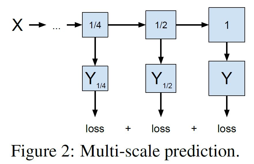
이미지 크기가 커질 수록, 정교하게 픽셀 레벨의 예측을 하는 것은 굉장히 어려워진다. Multi-scale 접근 방법은 Input에 대해 Multi-scale 이미지 피라미드를 형성하는 관점에서 사용되어 왔지만 Multi-scale Output 예측을 위해서는 잘 사용되지 않았다.

본 논문에서 우리는 다른 scale로 Output을 예측하는 네트워크를 학습시킬 것을 제안한다. 그렇게 함으로써, global-to-loca, coarse-to-fine-grained한 픽셀 레벨의 semantic label에 대한 예측을 수행할 수 있다. 위 그림은 3가지 scale로 학습을 진행하는 모습에 대한 예시이다.

1.4.3.2. Training with Input Omission Noise

깊은 신경망의 뉴런에 Noise를 추가하는 것은 대표적인 규제 방법 중 하나이다. 우리는 Semantic Segmentation에 대해서 간단한 규제 테크닉을 제안한다. Input 데이터 $\mathbf{x}$ 를 Noise Process에 따라 오염시켜 $\tilde{\mathbf{x}}$ 로 만들고 목적함수 $\tilde{\mathcal{L} (\mathbf{\tilde{x}, y})}$ 로 네트워크를 최적화하는 것이다.

Noise Process는 임의로 정할 수 있는데, 본 문제에서는 Random Block Omission Noise를 제안한다. 특히 우리는 이미지의 40% 이하의 면적에 대해 사각형의 마스크를 랜덤하게 생성하고, 그 부분의 픽셀 값을 0으로 만드는 방법을 사용하였다. 이는 Block 폐쇄 혹은 결측값을 시뮬레이션한 것으로, 예측 문제를 더욱 어렵게 만드는 요인으로 파악할 수 있다.

이렇게 제안된 전략은 또한 Denoising 학습 방법과 연관되어 있다고도 볼 수 있는데, 우리는 Input 데이터에만 Noise를 투사하고 Missing Input을 재구성하지는 않는다는 점이 다르다.

1.5. Experiments

(논문 원본 참조)

1.6. Conclusion

구조화된 Output 변수에 대해 복수의 Mode를 갖는 분포를 모델링하는 것은 구조화된 예측 문제에 대해 좋은 성과를 내는 데에 있어 중요한 이슈이다. 본 연구에서 우리는 가우시안 잠재 변수를 이용하여 Conditional Deep Generative Model에 근거한 확률적 신경망을 제안하였다.

제안된 모델은 scalable하며 추론과 학습에 있어 효율적이다. 우리는 Output 공간이 복수의 Mode를 갖는 분포에 대해 확률적인 추론을 하는 것의 중요성을 역설하였고, Segmentation 정확도, 조건부 Log Likelihood 추정, 생성된 Sample의 시각화 측면에서 모두 뛰어난 성과를 냈다는 것을 보여주었다.

2. Tensorflow로 확인

VAE를 다루었던 이전 글에서 크게 바뀐 부분은 없다.
본래 이 논문에 나와있는 내용에 충실히 따라서 구현을 해야겠지만… 이 논문 이후에 나온 다른 논문들에 더 집중하기 위해 본 글에서는 간단히 $y$ 를 Input으로 추가했을 때 어떤 효과가 나오는지 정도만 확인을 하도록 하겠다.

Convolutional 형태를 취했던 이전 모델과 달리 $y$ 를 Input으로 넣기 위해 모두 Flatten한 상태로 네트워크를 구성하였다. 이번에는 Label 데이터도 같이 불러온다.

train_dataset = (tf.data.Dataset.from_tensor_slices(
    (tf.cast(train_images, tf.float32), tf.cast(train_labels, tf.float32)))
                 .shuffle(train_size).batch(batch_size))
test_dataset = (tf.data.Dataset.from_tensor_slices(
    (tf.cast(test_images, tf.float32), tf.cast(test_labels, tf.float32)))
                .shuffle(test_size).batch(batch_size))

모델은 아래와 같다. encode, decode 단계에서 $y$ 가 Input으로 추가되어 있는 모습을 확인할 수 있다.

class CVAE(tf.keras.Model):
    def __init__(self, latent_dim):
        super(CVAE, self).__init__()
        self.latent_dim = latent_dim
        self.encoder = tf.keras.Sequential(
            [
                tf.keras.layers.InputLayer(input_shape=(28*28 + 1)),
                tf.keras.layers.Flatten(),
                tf.keras.layers.Dense(units=512, activation='relu'),
                tf.keras.layers.Dropout(rate=0.2),
                tf.keras.layers.Dense(units=256, activation='relu'),
                tf.keras.layers.Dropout(rate=0.2),
                tf.keras.layers.Dense(units=64, activation='relu'),
                tf.keras.layers.Dense(units=latent_dim + latent_dim),
            ])

        self.decoder = tf.keras.Sequential(
            [
                tf.keras.layers.InputLayer(input_shape=(latent_dim+1)),
                tf.keras.layers.Dense(units=64, activation='relu'),
                tf.keras.layers.Dropout(rate=0.2),
                tf.keras.layers.Dense(units=256, activation='relu'),
                tf.keras.layers.Dropout(rate=0.2),
                tf.keras.layers.Dense(units=512, activation='relu'),
                tf.keras.layers.Dense(units=784),
            ])

    @tf.function
    def encode(self, x, y):
        inputs = tf.concat([x, y], 1)
        mean, logvar = tf.split(self.encoder(inputs), num_or_size_splits=2, axis=1)
        stddev = 1e-8 + tf.nn.softplus(logvar)
        return mean, stddev

    def reparameterize(self, mean, stddev):
        eps = tf.random.normal(shape=mean.shape)
        z = mean + eps * stddev
        return z

    @tf.function
    def decode(self, z, y, apply_sigmoid=False):
        inputs = tf.concat([z, y], 1)
        logits = self.decoder(inputs)
        if apply_sigmoid:
            probs = tf.sigmoid(logits)
            return probs
        return logits

학습 및 테스트 코드는 아래와 같다.

optimizer = tf.keras.optimizers.Adam(1e-4)

def compute_loss(model, x, y):
    x = tf.reshape(x, [-1, 784])
    y = tf.reshape(y, [-1, 1])
    mean, stddev = model.encode(x, y)
    z = model.reparameterize(mean, stddev)
    x_logit = model.decode(z, y, True)
    x_logit = tf.clip_by_value(x_logit, 1e-8, 1-1e-8)

    # Loss
    marginal_likelihood = tf.reduce_sum(x * tf.math.log(x_logit) + (1 - x) * tf.math.log(1 - x_logit), axis=[1])
    loglikelihood = tf.reduce_mean(marginal_likelihood)

    kl_divergence = -0.5 * tf.reduce_sum(1 + tf.math.log(1e-8 + tf.square(stddev)) - tf.square(mean) - tf.square(stddev),
                                         axis=[1])
    kl_divergence = tf.reduce_mean(kl_divergence)

    ELBO = loglikelihood - kl_divergence
    loss = -ELBO

    return loss


@tf.function
def train_step(model, x, y, optimizer):
    with tf.GradientTape() as tape:
        loss = compute_loss(model, x, y)
    gradients = tape.gradient(loss, model.trainable_variables)
    optimizer.apply_gradients(zip(gradients, model.trainable_variables))

    return loss


epochs = 30
latent_dim = 2
model = CVAE(latent_dim)

# Train
for epoch in range(1, epochs + 1):
    train_losses = []
    for x, y in train_dataset:
        loss = train_step(model, x, y, optimizer)
        train_losses.append(loss)

    print('Epoch: {}, Loss: {:.2f}'.format(epoch, np.mean(train_losses)))


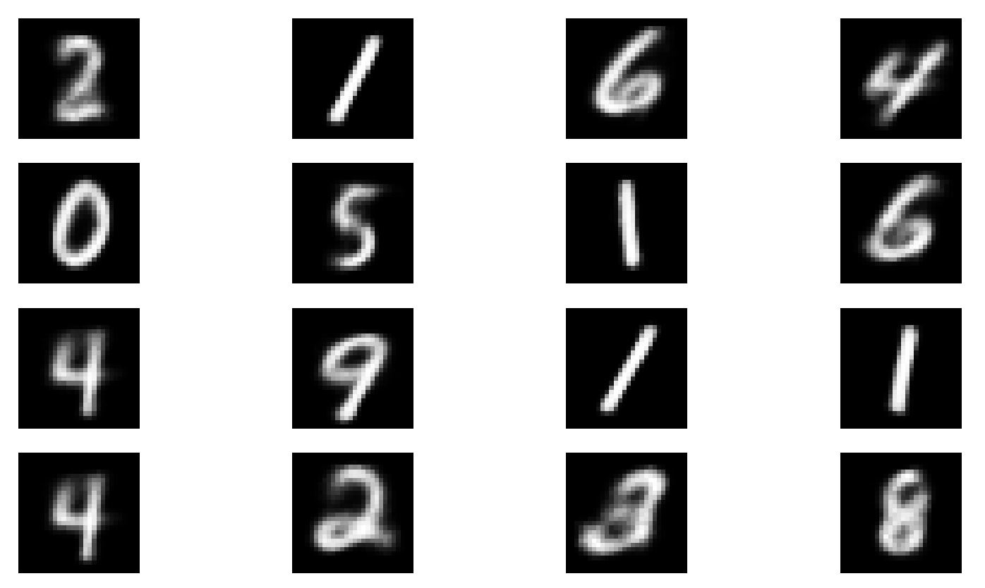
# Test
def generate_images(model, test_x, test_y):
    test_x = tf.reshape(test_x, [-1, 784])
    test_y = tf.reshape(test_y, [-1, 1])
    mean, stddev = model.encode(test_x, test_y)
    z = model.reparameterize(mean, stddev)

    predictions = model.decode(z, test_y, True)
    predictions = tf.clip_by_value(predictions, 1e-8, 1 - 1e-8)
    predictions = tf.reshape(predictions, [-1, 28, 28, 1])

    fig = plt.figure(figsize=(4, 4))

    for i in range(predictions.shape[0]):
        plt.subplot(4, 4, i + 1)
        plt.imshow(predictions[i, :, :, 0], cmap='gray')
        plt.axis('off')

    plt.show()


num_examples_to_generate = 16
random_vector_for_generation = tf.random.normal(shape=[num_examples_to_generate, latent_dim])
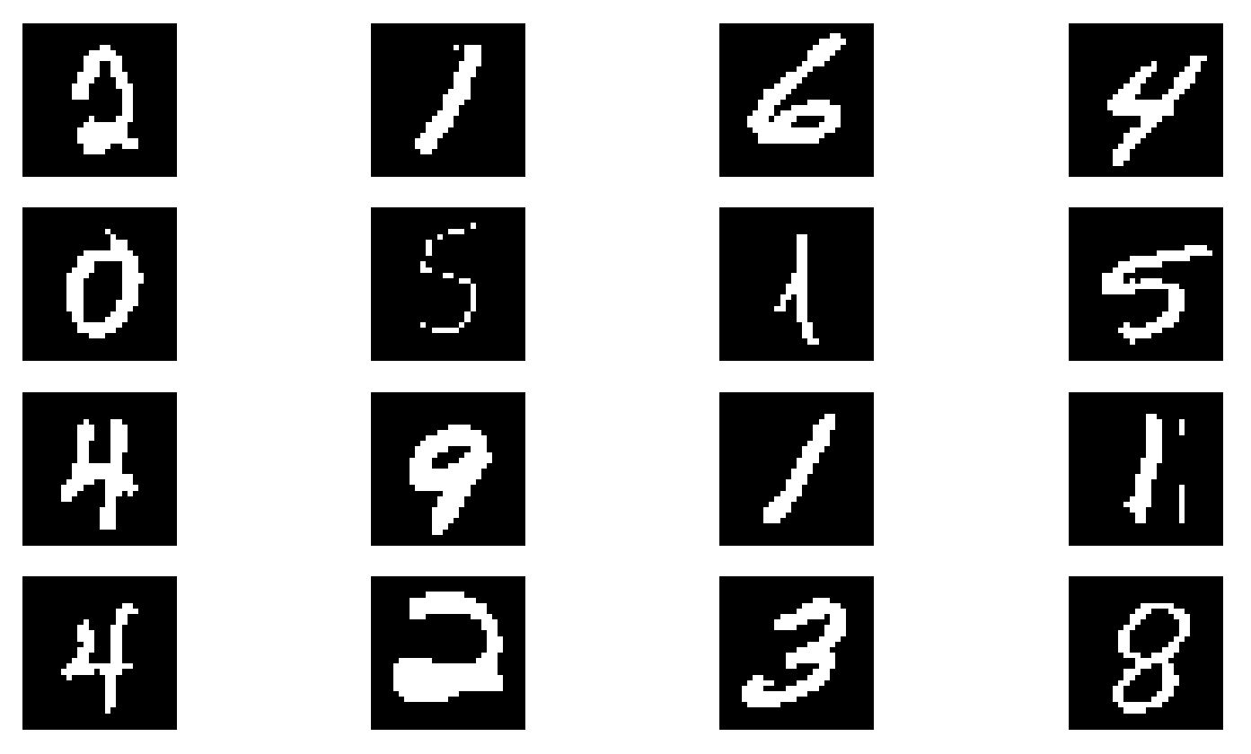
test_x, test_y = next(iter(test_dataset))
test_x, test_y = test_x[0:num_examples_to_generate, :, :, :], test_y[0:num_examples_to_generate, ]

for i in range(test_x.shape[0]):
    plt.subplot(4, 4, i + 1)
    plt.imshow(test_x[i, :, :, 0], cmap='gray')
    plt.axis('off')

plt.show()

generate_images(model, test_x, test_y)

VAE와 동일하게 Epoch 30이후의 결과를 확인하면 다음과 같다. 기존 이미지와 상당히 유사하게 새로운 이미지를 생성한 것을 확인할 수 있다. (Loss도 127까지 줄어들었다. 다만 좀 흐릿하긴 하다.)

Reference

논문 원본