Back to Basics: Let Denoising Generative Models Denoise | Summary

Contents

Summary
1. Introduction
2. Related Work
3. On Prediction Outputs of Diffusion Models
4. “Just Image Transformers” for Diffusion
5. Comparisons
6. Discussion and Conclusion
Appendix
Brief Thoughts

This article explains the key points of Back to Basics: Let Denoising Generative Models Denoise.

2025-11-17 (arXiv)
Li, Tianhong, He, Kaiming.
MIT
Paper
Github

Summary

Image generators that progressively remove noise can fail when Transformers process large patches of raw pixels. On ImageNet 256×256, directly predicting clean images achieves Fréchet Inception Distance on 50,000 generated images (FID-50K; lower is better) of 8.62, versus 372.38 for noise prediction and 96.53 for flow-velocity prediction, the prediction of the noisy sample’s rate of change, using the same base-size Just image Transformers model with 16×16 patches (JiT-B/16), velocity-space loss, 200 training epochs, and classifier-free guidance (CFG), which controls class conditioning during sampling.
JiT directly predicts clean images with a Vision Transformer (ViT), a Transformer operating on image patches, without a learned latent tokenizer, an encoder that maps pixels into a representation for generation, pre-training, or auxiliary losses. The reported comparisons use separately selected guidance settings and exponential moving average (EMA) decays, which determine how model parameters are averaged over training.
The explanation rests on the manifold assumption: natural images approximately occupy a low-dimensional structure within pixel space, whereas noise and flow velocity occupy the surrounding high-dimensional space. A controlled synthetic experiment and ImageNet ablations support the claim that clean-image prediction remains effective when the network compresses its input.
The largest JiT models achieve FID 1.82 at 256×256 and 1.78 at 512×512, with almost unchanged computation per forward pass because patch size increases with resolution. Several reference methods achieve lower FID, and the proposed extension to other natural-data domains is not tested.

1. Introduction

The introduction distinguishes x-prediction, directly predicting the clean image, from ε-prediction, predicting noise, and v-prediction, predicting a mixture of clean data and noise. Although these quantities can be converted into one another algebraically, a finite-capacity network may find their prediction tasks different: preserving high-dimensional noise requires information that denoising can discard.

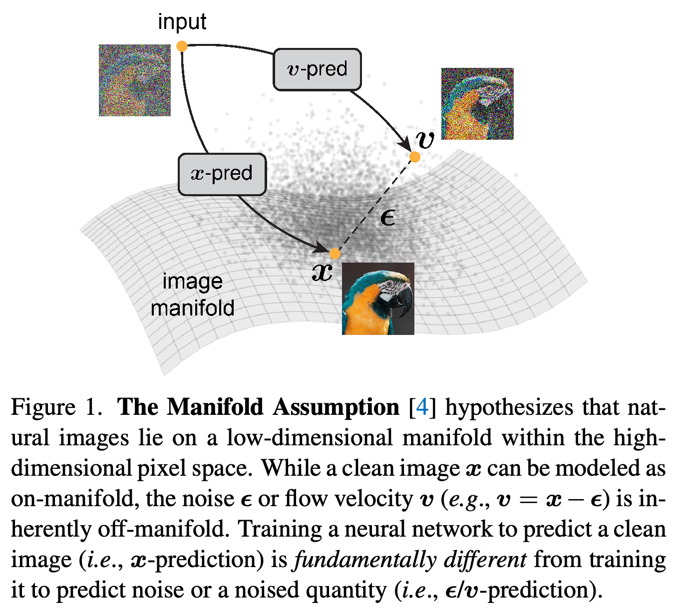
Figure 1 illustrates the proposed distinction between clean images on a low-dimensional manifold and noise-containing targets outside it.
JiT avoids a latent tokenizer, adversarial loss from a discriminator, perceptual loss based on a pre-trained classifier’s features, and representation alignment with a pre-trained model.
The proposed relevance to proteins, molecules, and weather is a motivation; the reported experiments use ImageNet.

Clean-image and velocity prediction targets relative to an assumed image manifold.

The related work connects diffusion prediction targets with classical denoising and manifold learning, the learning of low-dimensional representations from observations. Denoising Autoencoders (DAEs), networks trained to reconstruct clean inputs from corrupted versions, motivate this connection; Latent Diffusion Models (LDMs), models performing diffusion in an autoencoder’s representation space, reduce the observed dimensionality before generation.

Earlier pixel-space methods often preserve information through dense convolutions, expanded channels, skip connections that pass features across distant layers, or small initial patches. The authors suggest that these designs accommodate noise-containing prediction targets.
Elucidating the design space of diffusion-based generative models (EDM) wraps the network output in a pre-conditioner, a prescribed combination with the noisy input, so its network does not directly output the clean image.
Clean-image prediction predates JiT. The contribution is evidence that the direct output parameterization matters in high-dimensional settings.

3. On Prediction Outputs of Diffusion Models

The paper separates the prediction space, the quantity directly emitted by the network, from the loss space, the quantity used to compute training error. Choosing either from clean images, noise, or velocity produces nine formulations whose practical behavior can differ despite sharing algebraic conversions.

3.1. Background: Diffusion and Flows

Training interpolates between a clean image and noise using \(z_t = t x + (1-t)\epsilon\), with t in [0, 1]; the corresponding velocity is \(v=x-\epsilon\). Time follows a logit-normal distribution, meaning logit(t) is normally distributed, and generation integrates \(\frac{dz_t}{dt}=v_\theta(z_t,t)\) from noise at t = 0 to data at t = 1.

An ordinary differential equation (ODE), an equation specifying continuous change over time, defines the sampling trajectory.
The default numerical sampler is 50-step Heun, a numerical ODE solver; the network’s output can be converted to velocity before sampling.

3.2. Prediction Space and Loss Space

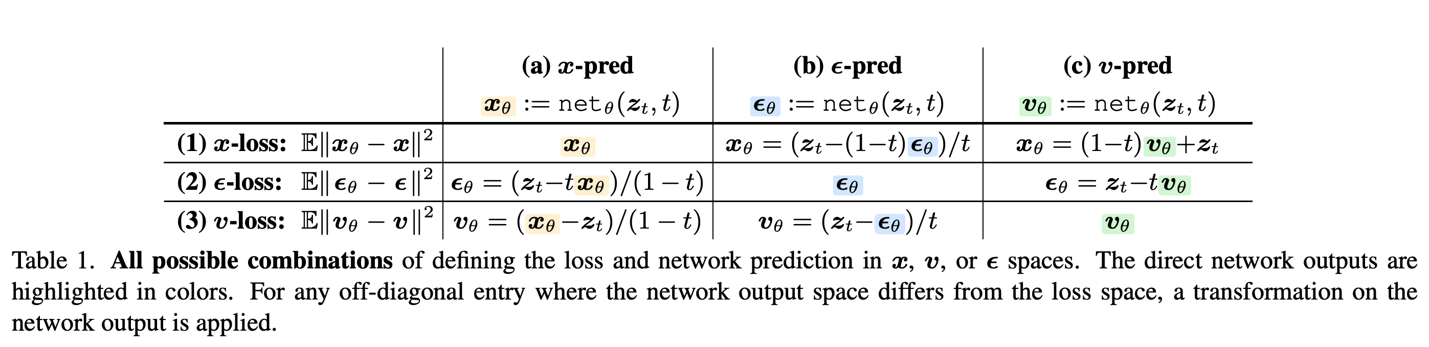
Table 1 enumerates all nine combinations of direct network output and loss space. For x-prediction, noise and velocity are recovered as \(\epsilon_\theta=\frac{z_t-tx_\theta}{1-t}\) and \(v_\theta=\frac{x_\theta-z_t}{1-t}\), allowing a clean-image output to be trained with a velocity-space loss.

With x-prediction, the v-loss becomes \(\mathbb{E}\left[\frac{\|x_\theta-x\|^2}{(1-t)^2}\right]\), a time-weighted clean-image reconstruction loss.
Changing the loss space changes the effective time weighting; changing the direct output also changes the task assigned to the network.
All nine formulations can generate samples after conversion to velocity, but the nine combinations of unweighted losses and direct outputs are not mathematically equivalent.

Conversions among clean-image, noise, and velocity outputs for three loss spaces.

3.3. Toy Experiment

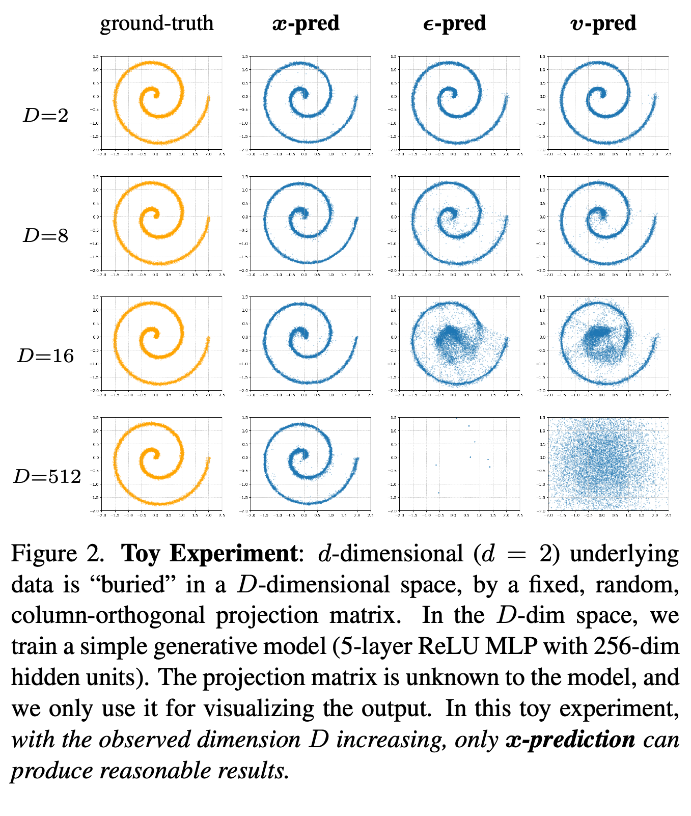
The toy experiment embeds two-dimensional spiral data into observed dimensions D ∈ {2, 8, 16, 512} using a fixed random column-orthogonal projection, whose columns are mutually orthonormal, unknown to the model. A five-layer multilayer perceptron (MLP), a stack of fully connected layers, with rectified linear unit (ReLU) activations and 256-dimensional hidden units learns generation using the same v-loss for each prediction target.

Figure 2 projects generated samples back to two dimensions for inspection: ε- and v-prediction deteriorate at D = 16 and fail at D = 512.
x-prediction preserves the spiral even at D = 512, where hidden width is smaller than observed dimension; this supports the capacity argument in a controlled synthetic setting.

Projected samples from a two-dimensional spiral embedded in higher-dimensional observation spaces.

4. “Just Image Transformers” for Diffusion

The image-generation experiments examine whether the synthetic experiment’s finding also holds for plain Transformers on raw pixels. The core proposal retains the standard patch-based architecture and makes its direct output the clean image.

4.1. Just Image Transformers

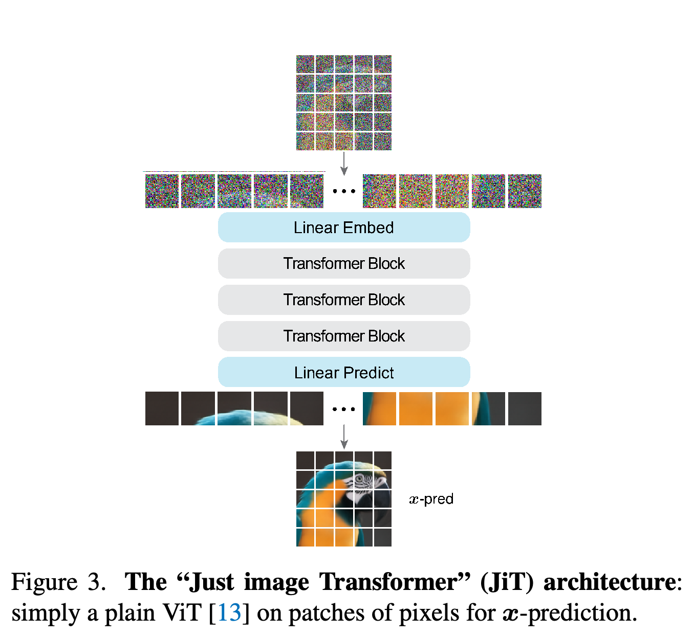
JiT splits a red-green-blue (RGB) image into non-overlapping p×p patches, linearly embeds each patch, adds positional information, processes the sequence with Transformer blocks, and linearly predicts clean output patches. Time and class labels condition the network through adaLN-Zero, the adaptive layer-normalization conditioning mechanism adopted from Diffusion Transformer (DiT).

Figure 3 shows the patch-to-patch architecture with linear input and output projections.
JiT/16 at 256×256 has 768 values per patch; JiT/32 at 512×512 has 3072. Both use a 16×16 patch grid, so their image-token sequence lengths are identical.

JiT architecture with patch embedding, Transformer blocks, and clean-image patch prediction.

4.2. What to Predict by the Network?

Table 2 tests all nine prediction/loss combinations using JiT-B with hidden width 768, 200 training epochs, and CFG, with guidance and EMA settings selected separately for each model. At 256×256 with 16×16 patches, x-prediction achieves FID 10.14, 10.45, and 8.62 under x-, ε-, and v-loss respectively; ε-prediction ranges from 372.38 to 394.58 and v-prediction from 96.53 to 126.88.

At 64×64 with 4×4 patches, patch dimension falls to 48 while hidden width and image-token sequence length remain unchanged; all nine combinations achieve FID between 3.46 and 6.20.
The comparison supports sensitivity to per-patch dimensionality and direct prediction target. Changing the loss space alone does not repair the tested high-dimensional failures.

FID-50K for nine output/loss combinations at two ImageNet resolutions after 200 epochs with CFG.

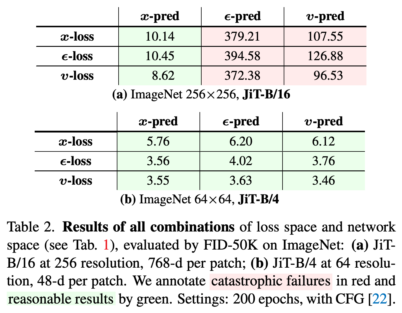
Table 3 varies the time-distribution mean μ to shift the training noise level. For x-prediction, FID improves from 14.44 at μ = 0.0 to 8.62 at μ = −0.8, then increases to 8.99 at μ = −1.2; ε- and v-prediction remain poor across the tested shifts.

The authors select μ = −0.8 for subsequent experiments.
Smaller μ produces smaller sampled times and more noise under the linear interpolation schedule. This adjustment improves x-prediction but does not resolve the tested failures of noise-containing outputs.

Effect of training noise-level shifts on JiT-B/16 FID-50K.

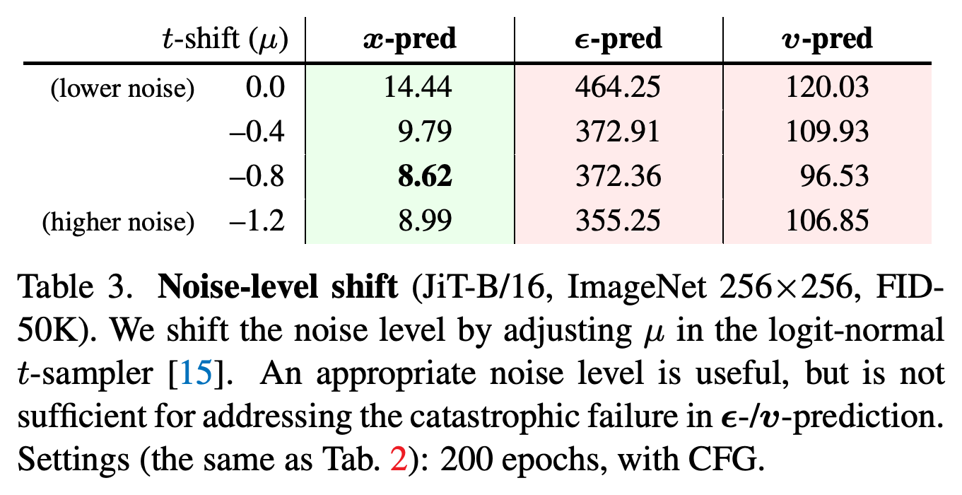
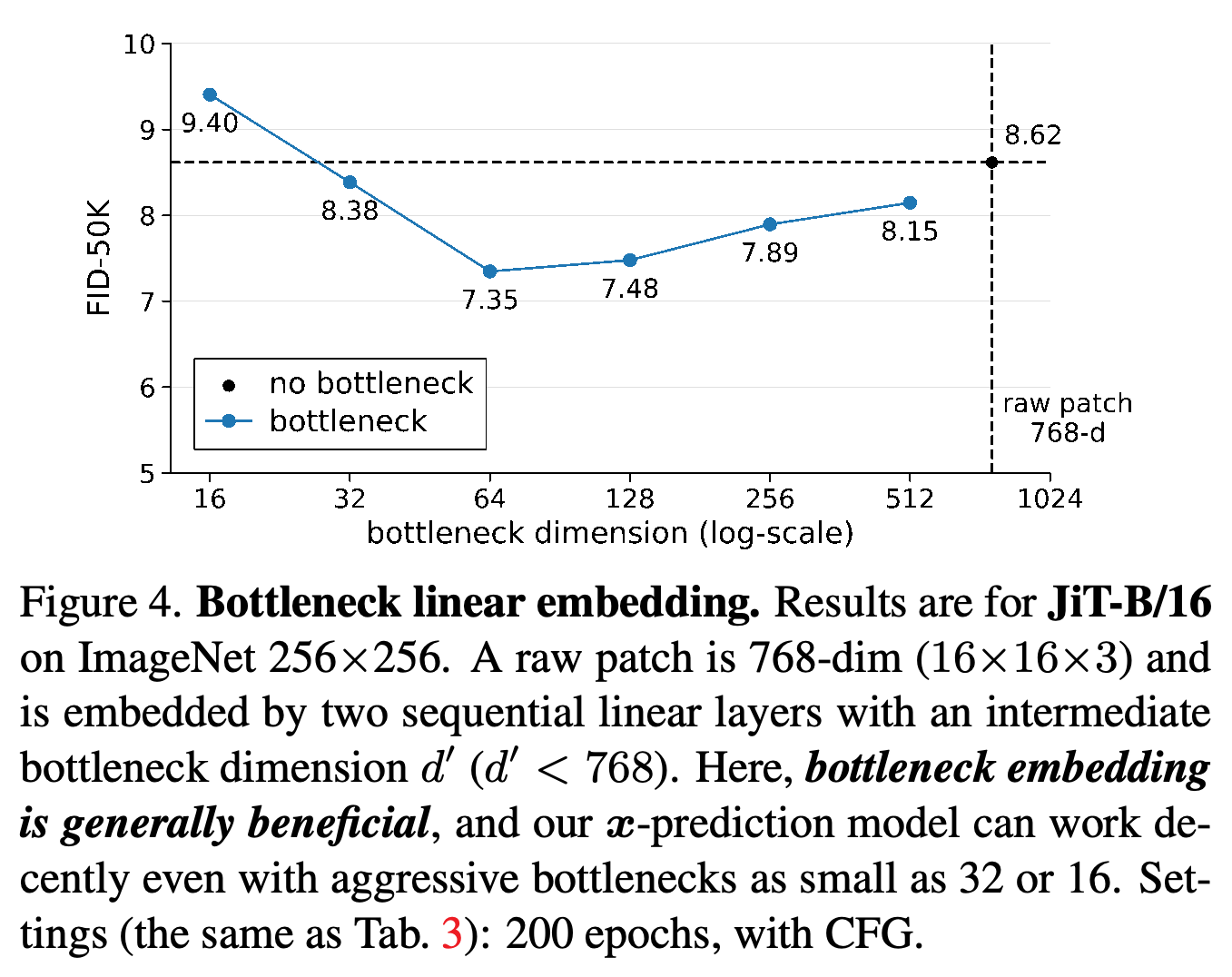
Figure 4 replaces the input projection with two linear layers whose intermediate dimension forms a bottleneck, a representation narrower than the raw patch. With JiT-B/16, a 64-dimensional bottleneck improves FID from 8.62 without a bottleneck to 7.35; even a 16-dimensional bottleneck yields 9.40 rather than catastrophic failure.

Intermediate dimensions 32, 128, 256, and 512 yield FID 8.38, 7.48, 7.89, and 8.15 respectively.
The experiment demonstrates that retaining every raw patch dimension is unnecessary for x-prediction; it does not directly measure the intrinsic dimension of natural images.

FID-50K versus input bottleneck dimension for JiT-B/16 on ImageNet 256×256.

4.3. Our Algorithm

The final algorithm directly predicts \(x_\theta=\operatorname{net}_\theta(z_t,t)\), converts it to \(v_\theta=\frac{x_\theta-z_t}{1-t}\), and minimizes expected squared velocity error. Algorithm 1 gives this training step, while Algorithm 2 updates a sample with z_next = z + (t_next − t) * v_pred using Euler integration, a numerical step along the predicted velocity.

The denominator 1 − t is clipped to a minimum of 0.05 whenever this division is computed.
The pseudocode omits class conditioning and CFG for brevity; the reported default sampler uses Heun rather than the illustrative Euler step.

4.4. “Just Advanced” Transformers

The advanced architecture uses SwiGLU, a gated Transformer component, RMSNorm, root mean square layer normalization, RoPE, rotary position embedding, and qk-norm, query-key normalization. It also uses 32 repeated class tokens with different positional embeddings as in-context conditioning, placing class information in the token sequence alongside the default adaLN-Zero conditioning.

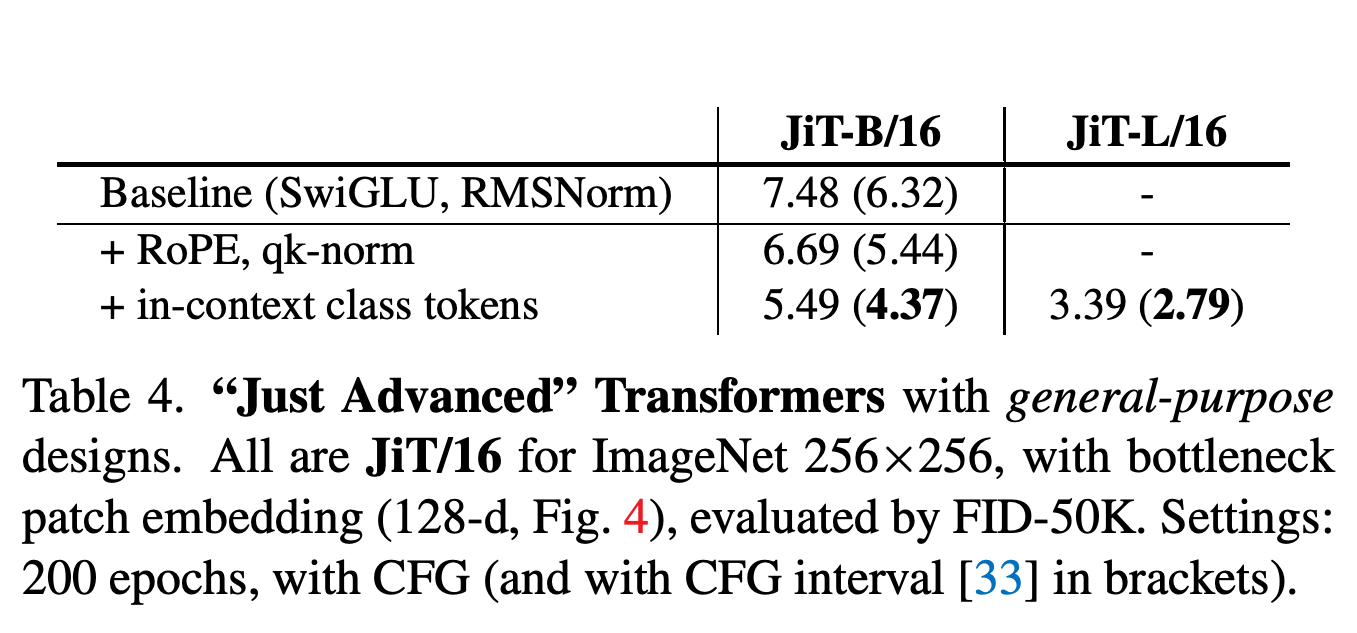
Table 4 uses a 128-dimensional input bottleneck and 200 epochs: JiT-B/16 improves from FID 7.48 with SwiGLU and RMSNorm to 6.69 with RoPE and qk-norm, then 5.49 with class tokens.
Restricting CFG to a sampling-time interval gives corresponding FID values 6.32, 5.44, and 4.37; JiT-L/16 achieves 2.79 with the complete design and interval.
The earlier ablations already include SwiGLU and RMSNorm. Table 4 therefore measures further architectural and guidance improvements beyond the basic x-prediction model.

Architecture and guidance-interval ablations for advanced JiT models.

5. Comparisons

Table 5 increases patch size in proportion to resolution, preserving 256 image tokens and JiT-B hidden width 768. At 256×256, 512×512, and 1024×1024, patch dimensions are 768, 3072, and 12288, while FID is 4.37, 4.64, and 4.82; model sizes are 131M, 133M, and 141M parameters, with 25, 26, and 30 Gflops, billions of floating-point operations, per forward pass.

Noise magnitude increases by 2× at 512 resolution and 4× at 1024; the remaining training recipe is preserved.
The similar costs concern models with different patch sizes, rather than a fixed-patch architecture applied to progressively longer image sequences.

JiT-B generation across three resolutions with proportional patch sizes.

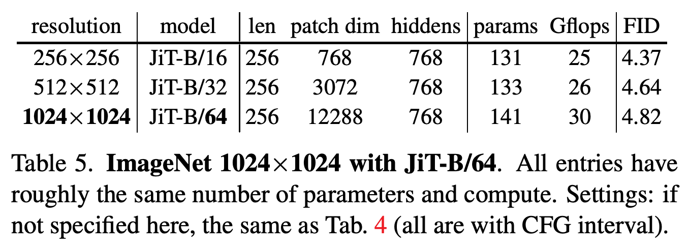
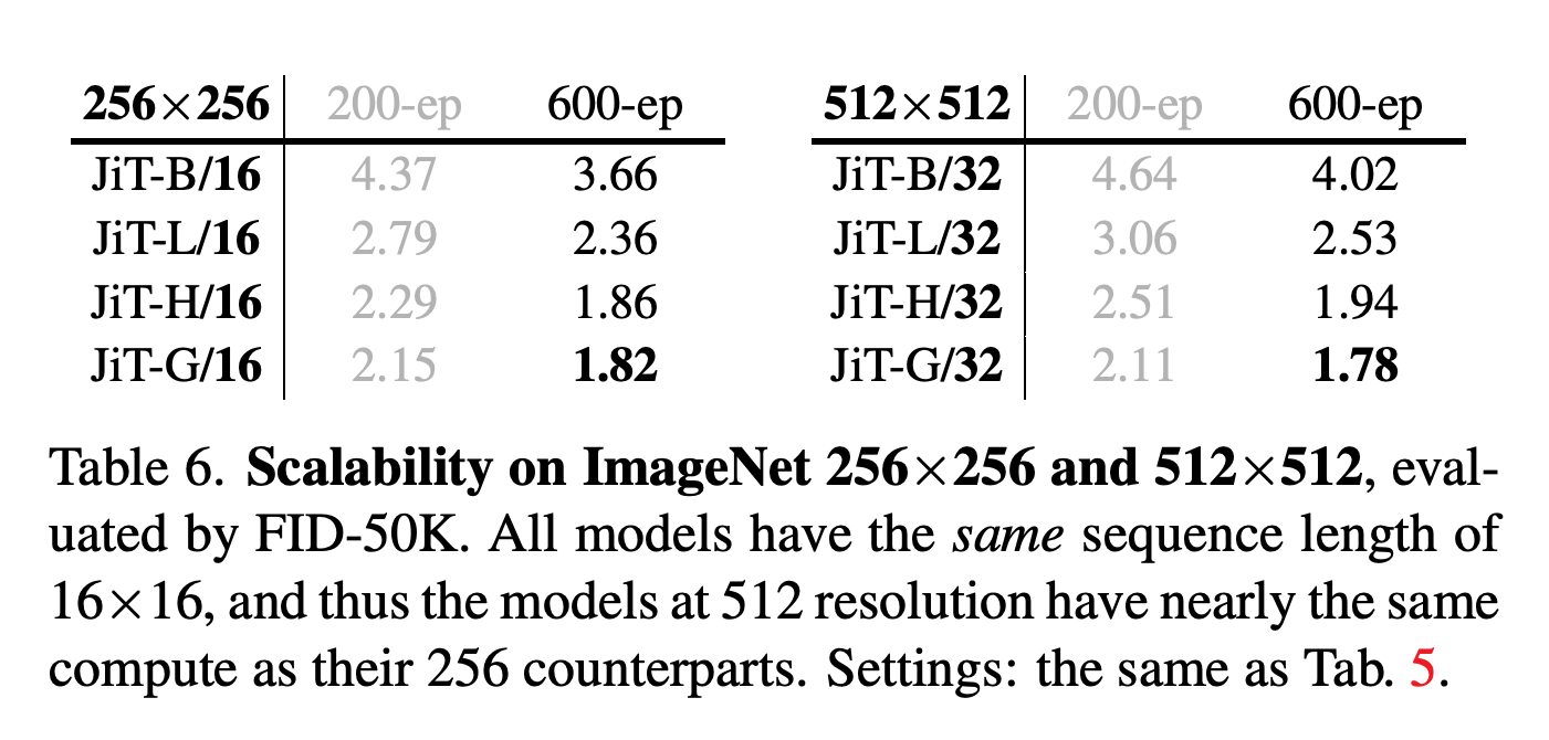
Table 6 shows improvements with model scale and longer training. In the columns labeled 600 epochs, JiT-B/L/H/G attain FID 3.66/2.36/1.86/1.82 at 256×256 and 4.02/2.53/1.94/1.78 at 512×512.

The appendix qualifies the training label: JiT-G models are stopped around 320 epochs when monitored FID begins to degrade.
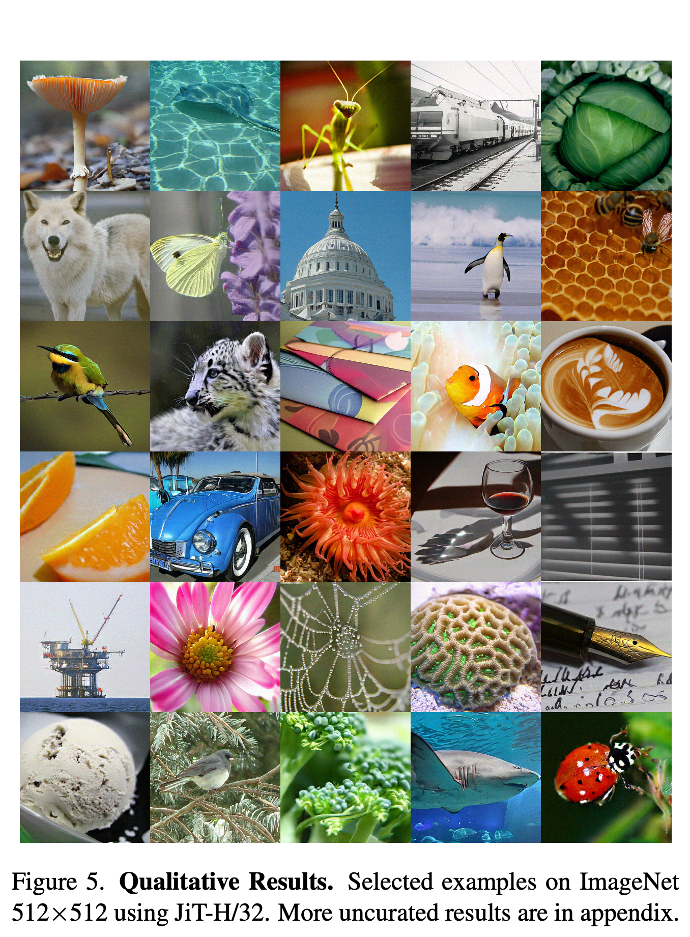
Figure 5 shows selected JiT-H/32 samples at 512×512, illustrating varied objects, textures, and scenes. The selected montage does not establish typical sample quality.

Model-size and training-duration scaling on ImageNet 256×256 and 512×512.

Selected ImageNet 512×512 samples generated by JiT-H/32.

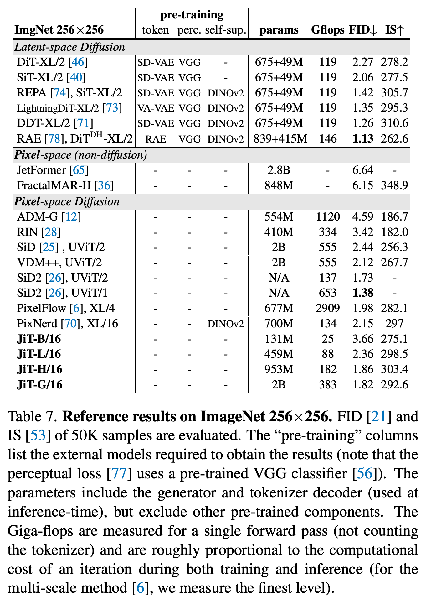
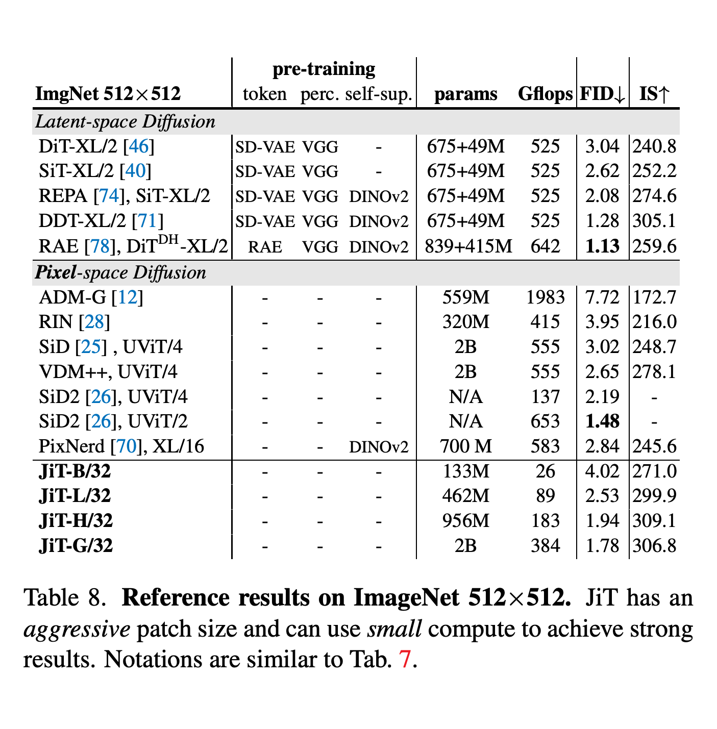
Tables 7 and 8 compare reference methods while identifying their pre-trained tokenizer, perceptual-loss, and self-supervised components, the latter trained without supervised labels. At 512×512, JiT-L/32 achieves FID 2.53 at 89 Gflops, versus SiT-XL/2, a scalable interpolant Transformer reference, at 2.62 and 525 Gflops; JiT-G/32 reaches 1.78 at 384 Gflops.

JiT does not achieve the lowest reference FID: at 512×512, Simpler Diffusion (SiD2) UViT/2 reports 1.48 at 653 Gflops, and the representation autoencoder (RAE) method, which generates in an encoded representation, reports 1.13 at 642 Gflops.
At 256×256, JiT-G/16 achieves 1.82 at 383 Gflops, while SiD2 UViT/2 reports 1.73 at 137 Gflops. The reference table therefore does not establish a universal compute advantage.
Gflops measure a single forward pass and exclude tokenizer computation; the comparisons do not match total training cost. The tables also report Inception Score (IS), an additional sample-quality score evaluated on the same 50K generated images.

ImageNet 256×256 reference results with pre-training dependencies, parameters, computation, FID, and IS.

ImageNet 512×512 reference results for latent-space and pixel-space diffusion methods.

6. Discussion and Conclusion

The conclusion emphasizes that neural-network capacity constrains prediction parameterizations: clean natural data and noise need not be equally tractable targets. JiT provides evidence for a diffusion-plus-Transformer design on raw images without external pre-trained components, while its suggested application to other high-dimensional natural data remains untested.

Appendix

A. Implementation Details: JiT-B/L/H/G use depths 12/24/32/40 and hidden dimensions 768/1024/1280/1664. Training uses the Adam optimizer with β₁ = 0.9 and β₂ = 0.95, batch size 1024, learning rate 2e-4, five warmup epochs, a constant learning-rate schedule, and zero weight decay; the time sampler uses μ = −0.8 and σ = 0.8. B/L use bottleneck width 128, H/G use 256, and H/G apply dropout 0.2, a training regularizer, in the middle half of the blocks; G models are stopped around 320 epochs when monitored FID worsens.
A. Implementation Details also specifies evaluation selection: CFG scales range from 1.0 to 4.0 in steps of 0.1, and EMA uses candidate decays 0.9996, 0.9998, and 0.9999. For each model, including each ablation, the authors choose settings using 8K generated samples, then evaluate 50K images against the ImageNet training set, with 50 samples for each of 1000 classes. Sampling uses 50 Heun steps and, when enabled, CFG interval [0.1, 1]; Figure 6 shows JiT-L/16 improving from best FID 2.88 without the interval to 2.36 with it.
B. Additional Experiments examines training errors, output pre-conditioning, an auxiliary classification objective, resolution transfer, and additional quality metrics. B.1. Training Loss and Denoised Images compares x- and v-prediction under the same v-loss: v-prediction has about 25% higher loss and visible single-step reconstruction artifacts in Figure 7. The text reports approximately 3× higher, unstable loss for ε-prediction and argues that reconstruction errors can accumulate during multi-step sampling.
B.2. Pre-conditioner tests x_θ = c_skip z_t + c_out net_θ(z_t, t), which mixes the noisy input with the network output using prescribed coefficients. Table 10 reports FID 28.94/72.05/35.49 for the adapted EDM-style formulation and 39.50/67.56/46.25 for a linear pre-conditioner under x-/ε-/v-loss, compared with direct x-prediction’s 10.14/10.45/8.62. The authors explicitly state that their noise schedule differs from EDM’s, so the adaptation is not fully equivalent to the original EDM formulation.
B.3. Exploration: Classification Loss attaches a pooled linear classifier after block 4 in JiT-B or block 8 in JiT-L and adds weighted cross-entropy, a classification loss, for the 1000 ImageNet classes. Class conditioning is disabled before the classifier to prevent label leakage, the classifier’s access to the target label through conditioning. At 200 epochs with CFG interval, Table 11 improves JiT-B/16 from FID 4.37 to 4.14 and JiT-L/16 from 2.79 to 2.50; this loss is excluded from the other experiments.
B.4. Cross-resolution Generation resizes generated images rather than changing the model’s native generation resolution. Downsampling JiT-G/32 outputs from 512 to 256 yields FID 1.84, close to native JiT-G/16’s 1.82; upsampling JiT-G/16 outputs to 512 yields 2.45, worse than native JiT-G/32’s 1.78. The authors attribute the latter degradation to missing higher-frequency detail.
B.5. Additional Metrics reports IS alongside generative precision and recall, measures of sample fidelity and distribution coverage. At 256×256, JiT-G/16 has IS 292.6, precision 0.79, and recall 0.62; SiT-XL/2 has 277.5, 0.82, and 0.59, while RAE has 262.6, 0.78, and 0.67. These results show differing fidelity and coverage profiles rather than uniform superiority on every metric.
C. Qualitative Results provides uncurated JiT-G/16 samples at 256×256 in Figures 8–11 across the specified animal, object, architectural, and natural classes. All four montages use CFG 2.2, the setting associated with reported FID 1.82, instead of a higher guidance value chosen specifically for visualization. The images supplement the aggregate metrics with examples of variation within classes.

Brief Thoughts

The strongest evidence is the separation of prediction target from loss space: Table 2 holds the architecture and evaluation procedure fixed across nine combinations, while selecting guidance and EMA settings for each model, and Figure 4 shows that substantial input compression remains compatible with effective clean-image prediction. Together with the synthetic projection experiment, these results support a capacity-sensitive explanation for the tested failures. The evidence does not prove that every high-dimensional diffusion model should use x-prediction; the low-dimensional settings in the paper work with all three targets. JiT is trained without external pre-trained components and has nearly constant forward-pass cost across the tested resolutions when patch size grows proportionally. FID gaps to stronger references, guidance and EMA selection, early stopping, and the absence of experiments beyond ImageNet limit broader claims.