


Regression Language Models for Code | Summary
30 Sep 2025 | Paper Review Code-to-Metric Regression Neural Architecture Search Multi-task RegressionContents
This article explains the key points of Regression Language Models for Code.
- 2025-09-30 (arXiv), 43rd International Conference on Machine Learning, PMLR 306, 2026
- Akhauri, Yash, Song, Xingyou, Wongpanich, Arissa, Lewandowski, Bryan, Abdelfattah, Mohamed S..
- Cornell University, Google DeepMind, Google Cloud
- Paper
- Github
Summary
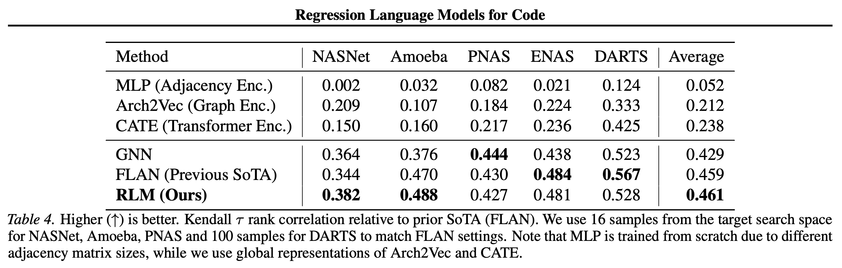
- Predicting execution memory, latency, and trained-network accuracy from code usually requires features tailored to each program or graph representation. The proposed Regression Language Model (RLM), which reads text and generates numeric targets, achieves average Kendall τ, a measure of ranking agreement, of 0.461 across five neural architecture search (NAS) spaces, sets of candidate network designs, compared with 0.459 for FLAN, the previous leading architecture predictor, under the reported target-space sampling settings.
- A roughly 300M parameter model uses a frozen T5Gemma encoder, a pretrained language model component that represents input text, and trains a decoder to generate numbers digit by digit. Constrained decoding restricts generation to valid numbers. Joint training covers high-level programs, Triton GPU kernels, programs compiled for graphics processors, and Open Neural Network Exchange (ONNX) text representations of neural-network computation graphs.
- The unified model reaches Spearman ρ, a correlation between predicted and observed rankings, of 0.930 on Python peak memory in APPS, a programming-problem dataset, and 0.516 on Triton kernel latency. Average ρ exceeds 0.5 across 24 languages in CodeNet, a multilingual code-submission dataset. It also outperforms GPT-5-Thinking in-context learning, prediction from labeled examples supplied in the prompt without updating model weights, across the four evaluated tasks.
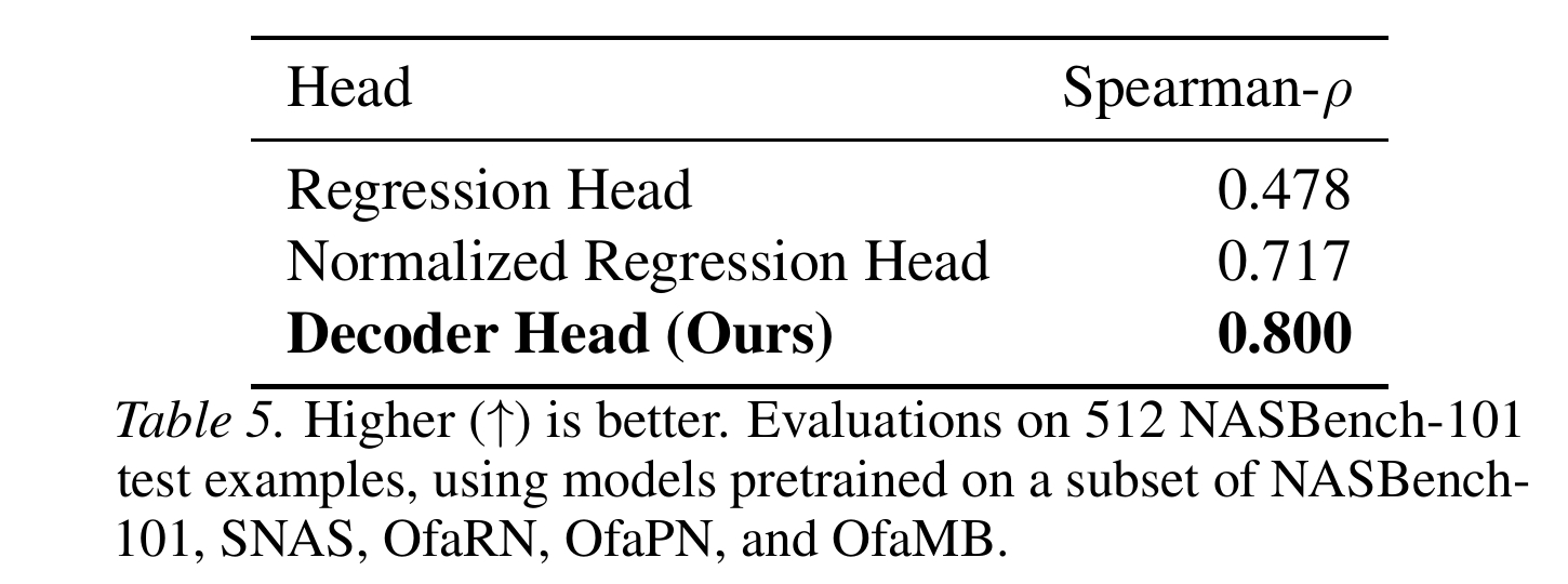
- In the output comparison, numeric decoding reaches ρ = 0.800, versus 0.717 for a normalized regression head, a component that predicts a scalar directly, and 0.478 for an unnormalized head. These comparisons match total layer count but allocate layers differently between encoding and decoding. Evaluation remains conditional on the data protocol: CodeNet training and testing share questions, latency uses specified hardware, and greater language diversity or fine-tuning, further training on a target task, does not reliably improve already well-represented code tasks.
1. Introduction
The paper defines code-to-metric regression as predicting numerical properties of a program or computation graph, such as memory consumption, execution latency, or accuracy after training. It asks whether a shared text-based predictor can reduce task-specific feature engineering while remaining competitive with graph neural networks (GNNs), models that learn from graph connectivity.
- Regression becomes next-token prediction over numeric outputs.
- The introduction identifies frozen language encoders, synthetic regression pretraining, numeric tokenization, and encoder context length as the principal design choices.
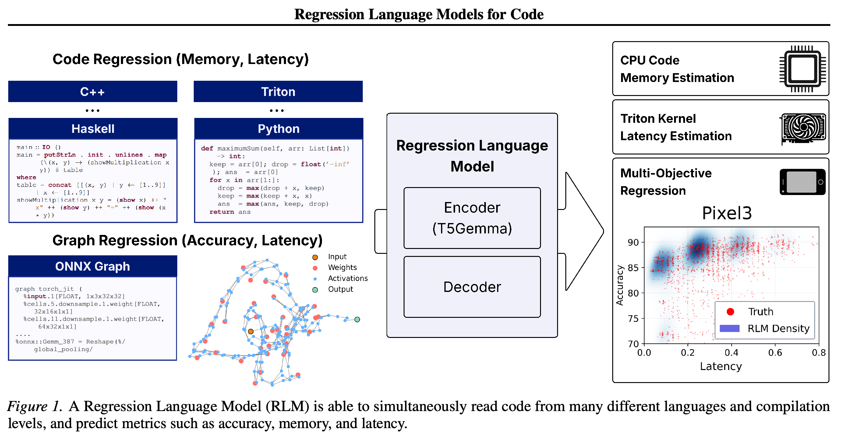
High-level source code and serialized neural-network graphs feed the same encoder–decoder, which emits different numeric metrics. The density illustration shows the intended joint-output interface rather than a separate benchmark result.
2. Related Work and Motivation
Earlier approaches summarize command counts, program statistics, syntax trees, graph paths, or hardware features before applying specialized predictors. Such representations can depend on a fixed operation vocabulary or graph format, requiring additional work when programs, kernels, or target metrics change.
- The paper distinguishes numeric generation from attaching a scalar regression head to a pretrained large language model (LLM).
- Its motivation is representational flexibility; the experiments test whether that flexibility preserves ranking performance.
3. Method
The encoder reads an input string x, and the decoder learns to generate its numeric target y. Following the RLM approach of Akhauri et al. (2025) and Song et al. (2024), freezing the pretrained T5Gemma encoder limits backward passes to the decoder and reduces training cost.
- Special sign, exponent, and mantissa tokens, the significant digits of a number, encode outputs digit by digit: <+><-><1><7><2><5> represents +10⁻¹ × 725 = 72.5.
- Constrained decoding produces valid numeric samples. Their mean or median gives a point estimate, and their distribution supports density estimation without target normalization.
3.1. Multi-task Regression
A shared textual input and numeric output format allows one model to train on multiple regression tasks. It can first learn from real or synthetic regression data and then adapt through fine-tuning.
- The authors argue that a broadly applicable string-based model may require more pretraining data than a specialized graph model with a stronger structural inductive bias, a built-in preference for graph relationships.
3.2. Multi-Objective Modeling
Autoregressive generation, in which each output depends on preceding outputs, allows later metrics to depend on earlier ones through p(y′ | y, x). Architecture latency and classification accuracy can therefore be modeled jointly rather than through outputs assumed independent given an encoder representation.
- The general conditional form is p(y⁽ᵏ⁾ | y⁽ᵏ⁻¹⁾, …, y⁽¹⁾, x) for k > 1.
- The experiments generate validation accuracy followed by latencies on four hardware platforms.
4. Data
The datasets combine executable high-level code with neural-network graphs serialized as text. Labels include measured execution properties, dataset-provided memory values, and architecture benchmark metrics; available inputs and supervision differ across datasets.
4.1. High-Level Programming Datasets
APPS contains 10K Python problems, 232.4K solutions, and 131.7K test cases; approximately 99K solutions execute successfully for profiling. KernelBook, a dataset pairing PyTorch programs with compiled Triton kernels, supplies 12,652 successfully executed kernels from 18.2K problems, profiled on a single NVIDIA A6000.
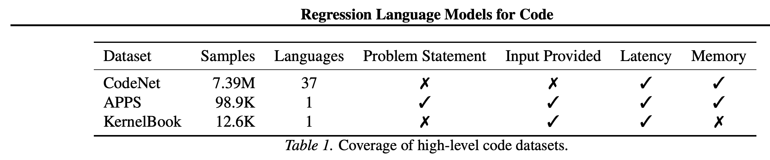
- CodeNet contains approximately 14M submissions in 37 languages. Filtering for accepted solutions yields approximately 7.3M entries, with 7.39M listed in Table 1; the target is its existing memory column.
- CodeNet lacks concrete program inputs. Training and test splits share questions, so evaluation concerns new submissions to previously observed questions rather than new-question zero-shot prediction, prediction without examples from the target question.
- The Triton kernels are produced by TorchInductor, the compiler used for the paired PyTorch programs. Most execution failures arise from the automated argument-matching harness rather than kernel correctness.
Input availability determines the evaluation conditions: CodeNet supplies neither problem statements nor concrete inputs, APPS supplies both, and KernelBook supplies inputs but no memory labels. The listed metrics describe dataset coverage rather than equally controlled prediction tasks.
4.2. NAS Datasets
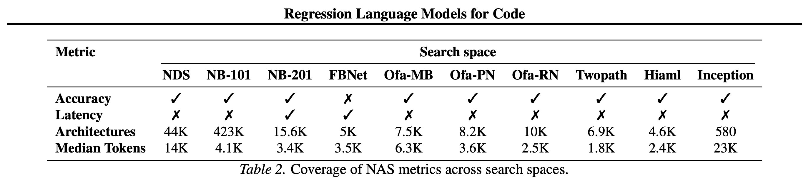
NAS prediction estimates architecture accuracy after training with fixed hyperparameters. The authors export architectures into ONNX intermediate representation (IR), a description of operations and connectivity, yielding approximately 520K unique architectures across the listed benchmark spaces.
- The collection includes NASBench-101, NASBench-201, FBNet, Once-for-all variants, Twopath, Hiaml, Inception, and Network Design Spaces (NDS).
- An additional author-created NAS space, SNAS, contains 85.5K architectures trained on CIFAR-10, an image-classification dataset, for 32 steps.
- Median serialized lengths range from 1.8K tokens for Twopath to 23K for Inception, making input truncation relevant.
Architecture spaces vary in size, available labels, and serialized length. Inception's 23K median tokens and NDS's 14K exceed the default 2048-token encoder limit, linking dataset coverage to input truncation and tokenizer design.
5. Experiments
The main model is jointly trained on the training splits of the code and architecture datasets. Experiments assess in-context regression, high-level code prediction, architecture ranking, and multi-objective prediction.
- Appendix A.3 compares code-only training with code-plus-graph training, and Appendix C gives default training and inference settings.
5.1. In-context Regression with LLMs
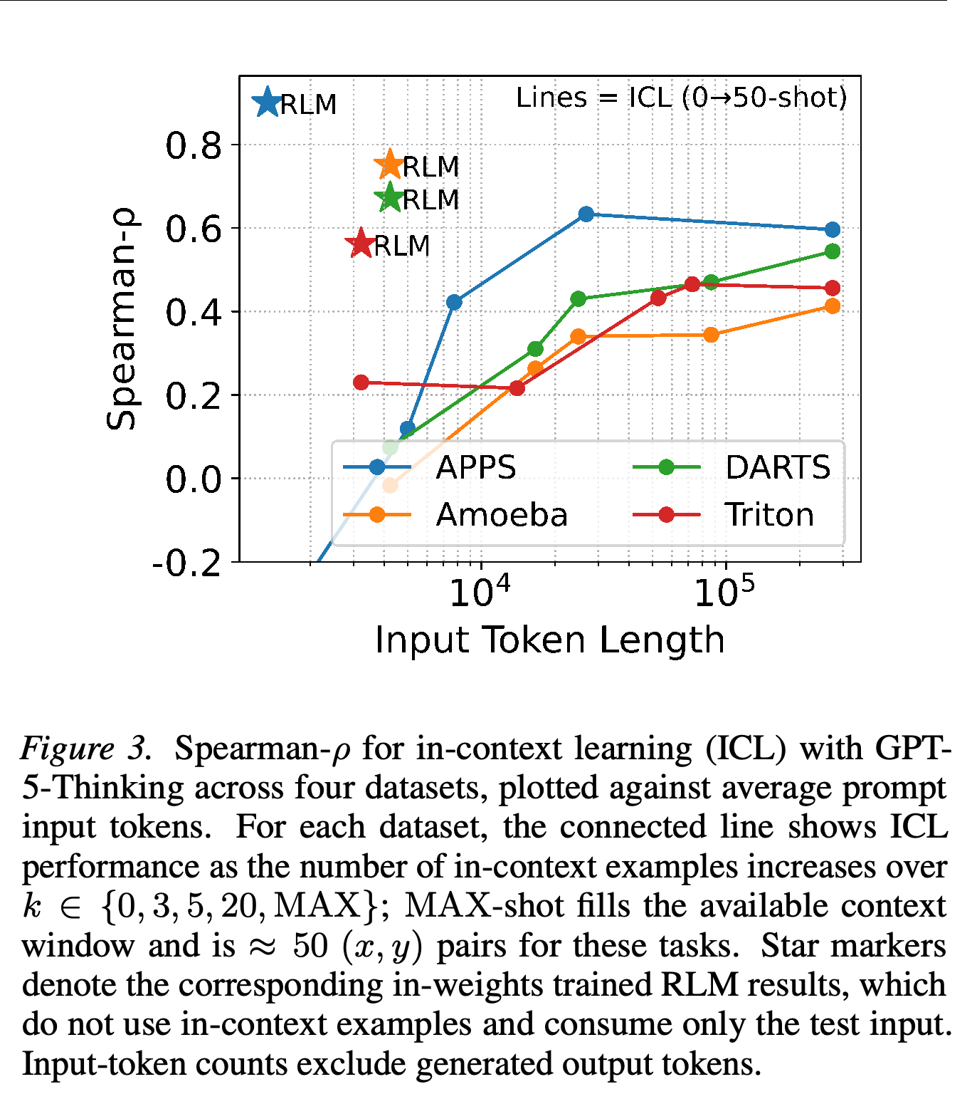
GPT-5-Thinking receives randomly sampled labeled examples followed by a test input, with k ∈ {0, 3, 5, 20, MAX}; MAX fills the context window with approximately 50 examples. Across APPS, Amoeba, DARTS, and Triton, adding examples generally improves in-context regression, but every reported setting remains below the trained RLM.
- MAX-shot prompts require approximately 2.7 × 10⁵ input tokens per query, compared with typically 10³–10⁴ tokens for the RLM’s raw test input in this comparison; generated output tokens are excluded. Appendix C separately specifies a default encoder limit of 2048 tokens.
- The paper estimates approximately $0.3125 per MAX-shot query, excluding thinking and output costs, and reports 12.5 RLM queries per second on a rented A6000. Its cost comparison depends on the stated pricing and deployment assumptions.
- The supervision budgets differ: the RLM learns from training examples, while GPT-5-Thinking receives only examples that fit in its prompt.
Adding prompt examples generally improves GPT-5-Thinking's ranking correlation while increasing input-token use. The trained RLM markers exceed all displayed prompt-based settings on the four tasks, although the models receive different training and inference supervision.
5.2. High-Level Programming Languages
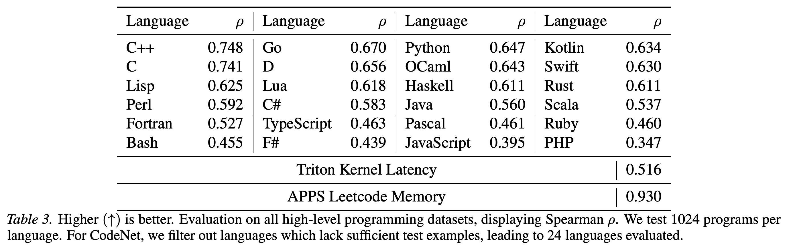
Table 3 evaluates 1024 programs per language and retains 24 CodeNet languages with sufficient test examples. Correlations range from ρ = 0.748 for C++ to 0.347 for PHP; APPS peak memory reaches 0.930 and Triton latency reaches 0.516.
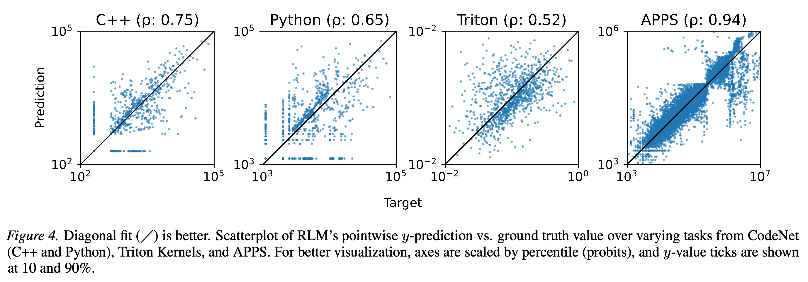
- The point-prediction plots span widely different target scales, but rank correlation does not measure absolute prediction error.
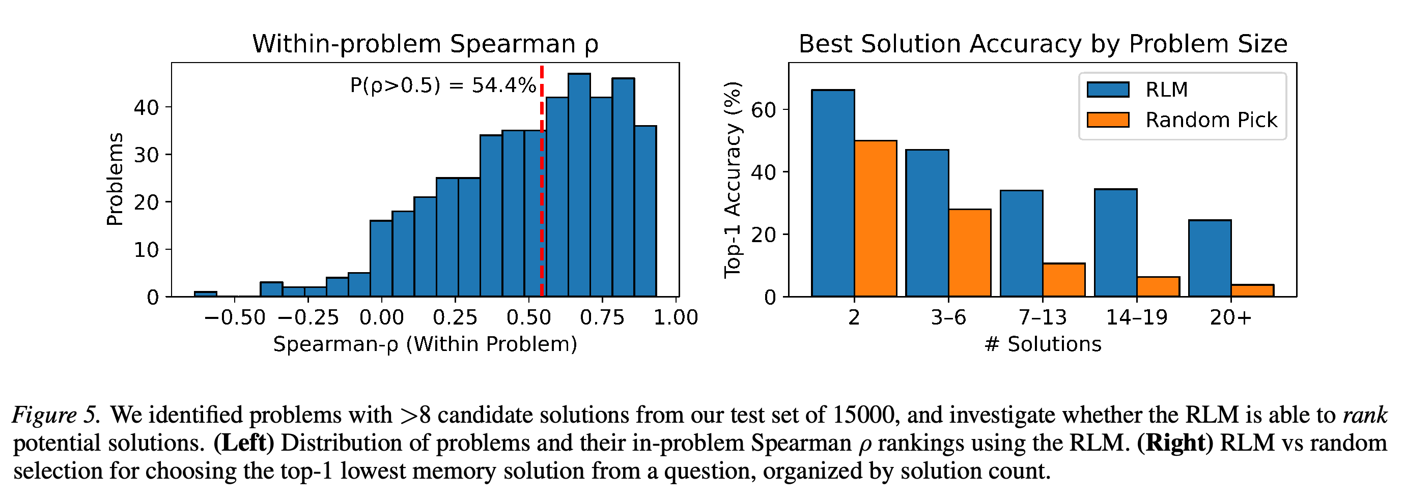
- The Figure 5 histogram reports within-problem ρ > 0.5 for 54.4% of the plotted problems. Selecting the predicted lowest-memory submission beats random selection across the displayed solution-count groups.
- The five worst-ranked APPS problems have a median coefficient of variation, target standard deviation divided by its mean, of approximately 0.0056 versus 0.037 for the five best. This associates nearly tied target values with poorer ranking.
The 24 language results show uneven ranking quality, from C++ at 0.748 to PHP at 0.347. APPS memory at 0.930 is substantially stronger than Triton latency at 0.516, so the shared interface does not imply uniform performance.
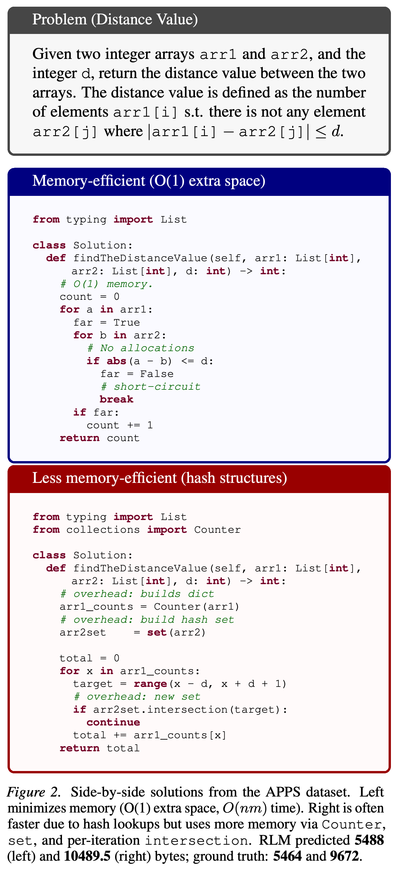
The predictor distinguishes a nested-loop implementation from one using Counter, set, and intersection allocations. Predictions of 5488 and 10489.5 bytes preserve the ordering of measured memory, 5464 and 9672 bytes, while showing different numerical errors for the two implementations.
Predictions track targets more tightly on APPS than on the other displayed tasks. The axes use percentile-based probit scaling, which maps percentiles to a normal-distribution scale, rather than directly displaying absolute error. The APPS panel reports 0.94, differing from Table 3's 0.930; the source does not explain the difference.
The histogram reports 54.4% of problems above within-problem ρ = 0.5. The bars show that selecting the predicted lowest-memory solution beats random selection in every displayed candidate-count group. The caption's more-than-eight-candidate condition does not describe all groups shown in the right panel.
5.3. NAS Results
Across NASNet, Amoeba, PNAS, ENAS, and DARTS, the RLM achieves average Kendall τ = 0.461, compared with 0.459 for FLAN and 0.429 for the GNN baseline. It leads on NASNet and Amoeba, while other methods lead on the remaining spaces.
- Table 4 specifies 16 target-space samples for NASNet, Amoeba, and PNAS, and 100 for DARTS to match FLAN settings. Its caption does not specify the ENAS sample count.
- The RLM uses ONNX text without FLAN’s additional zero-cost proxies, inexpensive architecture signals computed without full training (Akhauri & Abdelfattah, 2024b; Abdelfattah et al., 2021).
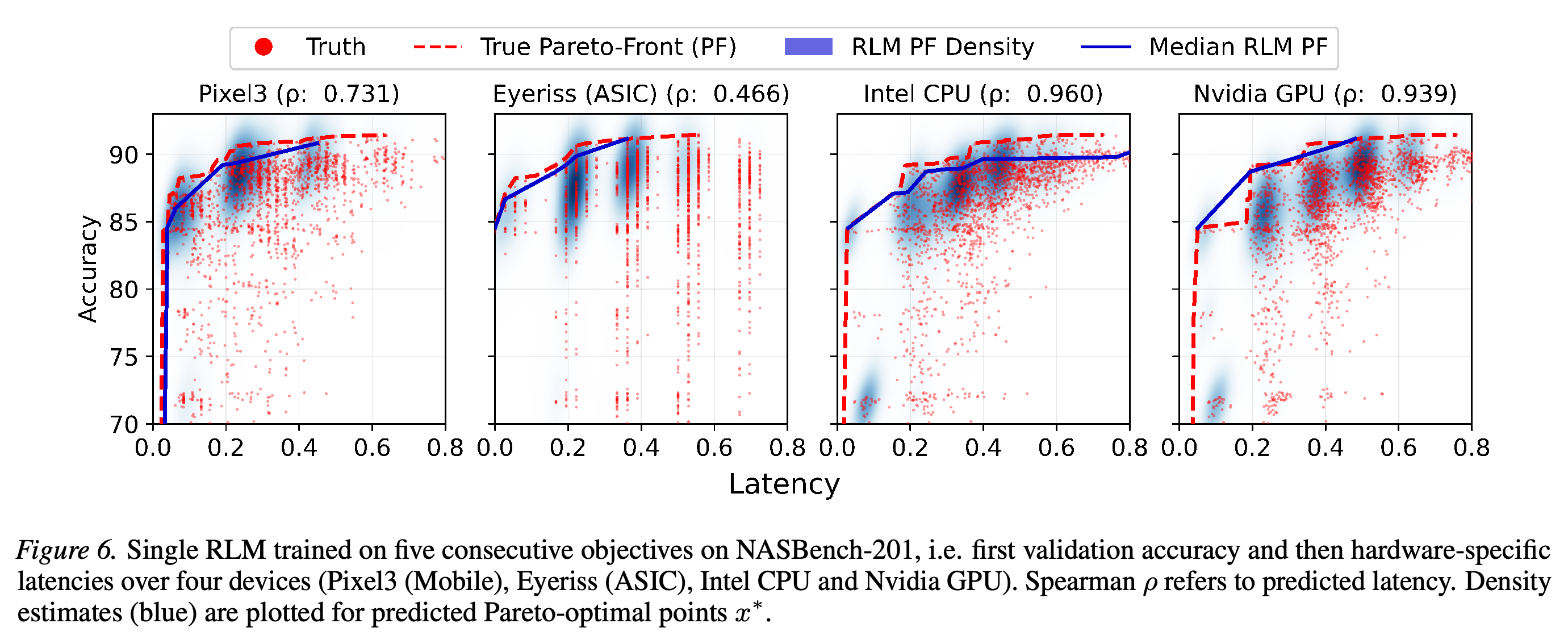
- A single NASBench-201 model generates accuracy and four device latencies. Latency correlations are 0.731 for Pixel3, 0.466 for Eyeriss, a specialized hardware accelerator, 0.960 for Intel CPU, and 0.939 for Nvidia GPU; predicted Pareto fronts, tradeoffs where improving one objective requires worsening another, broadly follow the observed fronts.
The RLM's average Kendall τ of 0.461 narrowly exceeds FLAN's 0.459. It leads on NASNet and Amoeba but trails the best method on PNAS, ENAS, and DARTS; no uncertainty estimates are supplied for the aggregate difference.
Predicted accuracy–latency fronts broadly follow measured tradeoffs, and the density contours show dependence between the generated metrics. Latency ranking varies by device, from 0.466 for Eyeriss to 0.960 for Intel CPU; these plots do not quantify uncertainty calibration.
6. Experiments: Ablations
The main ablations, controlled comparisons of design choices, examine numeric output generation, encoder size, and tokenization. They use different subsets and training conditions, so each result applies to its own comparison.
6.1. Comparing with Regression Heads
The output-head comparison holds total depth at four layers: a two-layer encoder plus two-layer decoder trained with cross-entropy, a loss on predicted token probabilities, versus a four-layer encoder with a mean squared error (MSE) regression head, a loss on squared numeric errors. On 512 NASBench-101 test examples, numeric decoding achieves ρ = 0.800, compared with 0.717 after per-dataset target normalization to [0, 1] and 0.478 without normalization.
- The training mixture includes NASBench-101, SNAS, and Once-for-all variants with substantially different target scales.
- The result supports the tested decoder design but does not isolate output representation from the allocation of layers between encoding and decoding.
Target normalization raises the regression-head correlation from 0.478 to 0.717. Numeric decoding reaches 0.800 in the matched-total-depth comparison, which also changes how layers are divided between encoding and decoding.
6.2. Scaling Regression Language Models
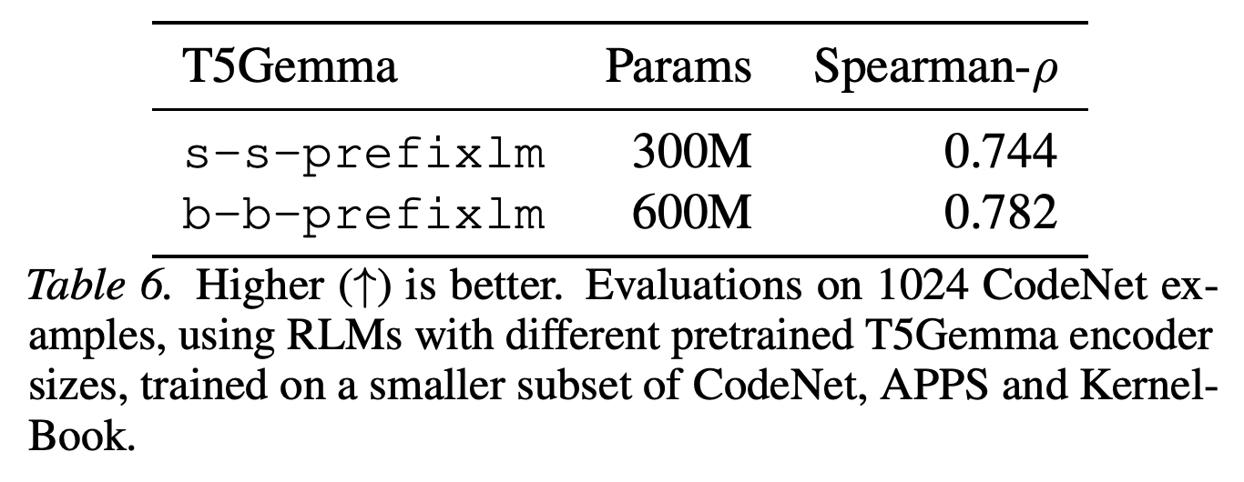
Replacing the smaller frozen encoder with t5gemma-b-b-prefixlm increases the model from 300M to 600M parameters. On a smaller mixed-code training subset and a 1024-example CodeNet evaluation, Spearman ρ improves from 0.744 to 0.782.
- The authors could not extend the comparison to larger T5Gemma models under their compute budget because those models required extensive hyperparameter tuning.
The 600M model improves correlation by 0.038 over the 300M model in the reported subset experiment. This two-size comparison demonstrates a local improvement but does not establish a broader scaling relationship.
6.3. Encoder-Decoder Settings
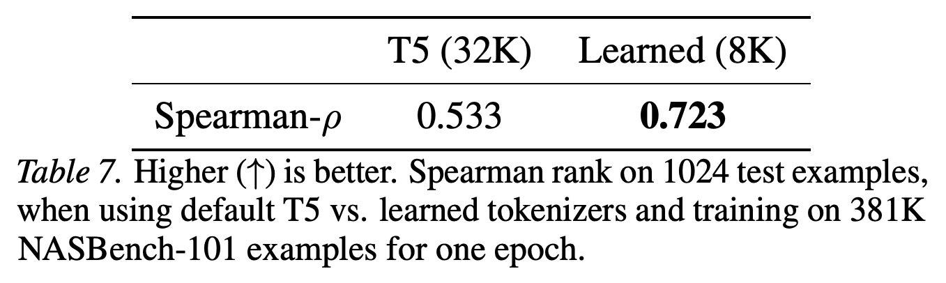
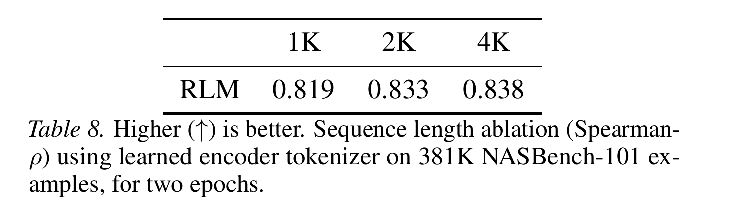
For models trained from scratch, an ONNX-aware SentencePiece tokenizer, a learned text segmentation vocabulary, uses 8K tokens and improves ρ from 0.533 with the default 32K-token T5 vocabulary to 0.723 after one epoch on 381K NASBench-101 examples. With the learned tokenizer and two epochs, increasing context from 1K to 2K to 4K raises ρ from 0.819 to 0.833 to 0.838.
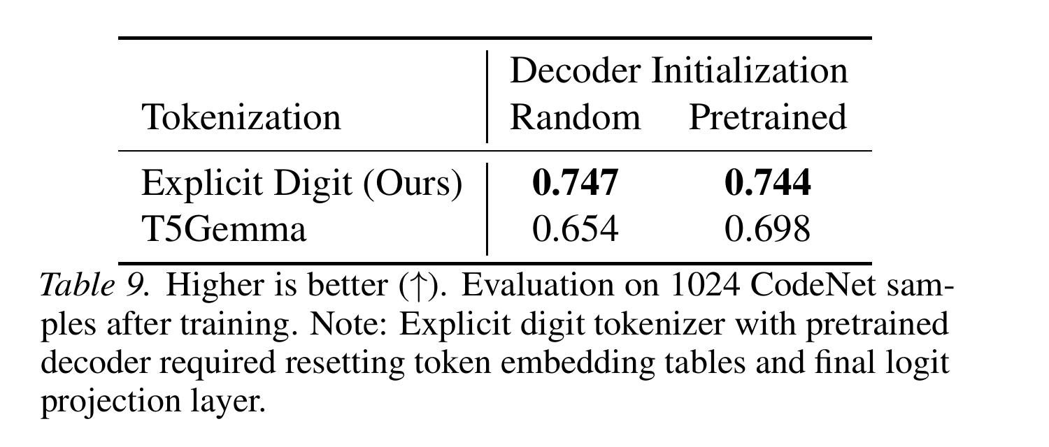
- Explicit numeric tokens achieve 0.747 with random decoder initialization and 0.744 with pretrained initialization; the standard T5Gemma tokenizer achieves 0.654 and 0.698, respectively.
- Decoder pretraining provides little observed benefit for the specialized numeric vocabulary, while the standard text vocabulary benefits from pretrained decoder weights.
- Using explicit numeric tokens with a pretrained decoder requires resetting its token embeddings and final output projection.
The 8K vocabulary learned from ONNX text yields 0.723 versus 0.533 for the default 32K T5 vocabulary after one epoch. The result supports adapting text segmentation to graph syntax when training from scratch.
Longer context improves correlation from 0.819 at 1K to 0.838 at 4K, with most of the gain occurring by 2K. The comparison shows a modest truncation-related effect for this tokenizer, dataset, and two-epoch training condition.
Explicit numeric tokens perform similarly with random and pretrained decoder initialization, while the standard tokenizer improves with pretrained initialization. Resetting embeddings and the final projection for explicit tokens is part of the comparison condition.
7. Conclusion
The paper concludes that numeric generation can provide a shared regression interface for multiple programming languages and computation-graph representations. It proposes applications in program search, hardware–software co-design, and compiler optimization; predicting the outcomes of entire experiments from raw code remains an open question.
Impact Statement
The authors state that the work aims to advance machine learning and identify no particular societal consequence requiring discussion. The statement includes no additional empirical analysis of downstream impacts.
Appendix
- A. Unified Model Ablations — A.1. Decoder-only Regressors: Qwen and Llama compares Qwen3-0.6B and Llama-3.2-1B, models that process inputs and generate outputs through a single decoder, using their default text tokenizers. Training uses 128K CodeNet, 80K APPS, and 10K KernelBook examples, 1024-token contexts, and roughly half the decoder layers frozen. Despite taking the median of 128 parsed generations, APPS memory correlations are approximately 0.15 and 0.17, respectively, versus approximately 0.90 for the T5Gemma RLM with P10, its dedicated numeric vocabulary. Frequent nonnumeric outputs motivate numeric constraints, although the comparison also changes backbone, tokenizer, and context conditions.
- A.2. Value of Pretraining distinguishes initialization from language training from prior training on regression tasks. T5Gemma initialization improves Triton correlation from 0.504 to 0.532. Pretraining on the synthetic FLOPs architecture metric, a measure of floating-point computation, reaches ρ = 0.999 on 1024 test architectures and improves subsequent accuracy prediction from approximately 0.83 to 0.85. The validation curves show faster convergence under both forms of pretraining.
- A.3. Training on Code and NAS compares code-only training with a code-plus-graphs mixture on 1024 examples per language. Average correlation changes from 0.701 to 0.706, with individual tasks moving in both directions; KernelBook training curves remain similar. These results support joint training without a large average loss in the tested mixture.
- A.4. Pretraining Diversity and Impact on Language fixes the total at 482K examples, including 15K examples each for Go, Haskell, and Rust, while varying the other 437K examples across one, two, four, or six languages. Table 11 averages are 0.45, 0.45, 0.37, and 0.43, respectively, with no monotonic benefit from language diversity. Go, Haskell, and Rust are represented during training; the table separately evaluates languages absent from the regression training mixture. The explanation that problem diversity matters more than syntax diversity is an author hypothesis.
- A.5. Fine-tuning reports that 1024 language-specific examples reduce correlation on all ten displayed code tasks, including C++ from 0.730 to 0.595 and Python from 0.637 to 0.448. Further training on approximately 1K target NAS examples improves NASBench201 from 0.681 to 0.738, NASBench101 from 0.646 to 0.734, ENAS from 0.165 to 0.516, and Amoeba from 0.045 to 0.501. The authors hypothesize catastrophic forgetting, degradation of previously learned abilities during further training, for the code results; they do not directly test that mechanism.
- B. Additional Experiments — B.1. Limited Information Scenario reports correlation decreasing from 0.93 with problem-plus-code input to 0.85 with code alone. B.2. Ranking measures whether the predicted best submission falls within the true top-p% for problems with more than eight solutions; its curve exceeds random selection. Appendix B describes these experiments using latency terminology, whereas Figure 5 and the principal APPS analysis emphasize memory, leaving the target interpretation inconsistent within the source.
- C. Experimental Settings uses https://github.com/google-deepmind/regress-lm and Adafactor, the training optimizer. Default learning rates are 1 × 10⁻³ for pretraining and 5 × 10⁻⁵ for fine-tuning, with gradient clipping at global norm 2.0, 10% linear warmup, and cosine decay. Unless matching a specified T5Gemma decoder, the model uses two decoder layers with hidden sizes 2048 and eight attention heads. Point estimates take the median of 64 decoder samples, and the default encoder truncates inputs beyond 2048 tokens; the authors report truncation only for ONNX graphs.
- D. Data: Extended — D.1. y-Value Distributions shows heterogeneous memory and latency targets that motivate normalization-free numeric decoding. D.2. Extra Leetcode Data for APPS adds 600 EffiBench examples, another collection of programming problems and submissions, and measures repeated wall-clock execution on cases supplied by generate_test_case(). D.3. Generating the SNAS Dataset samples lightweight convolutional neural networks, image models built from convolution operations, and briefly trains them on CIFAR-10 using stochastic gradient descent with momentum, cosine learning-rate scheduling, and mixed precision, computation using FP16/BF16 formats. Each architecture is recorded with accuracy, training, and architecture metadata.
- D.4. Hardware Profiling — D.4.1. APPS uses an AMD EPYC 7702, 503 GiB RAM, Ubuntu 22.04, and Linux 6.8.0-45-generic. Each run executes in a fresh Python process with -I -S -B; the default timing protocol discards three warmups, measures eleven repeats, and applies a 10 s timeout. The primary memory target is dyn_peak_alloc_bytes collected in a separate untimed run with tracemalloc, a Python allocation tracer. It measures Python-heap usage rather than total process memory.
- D.4.2. KERNELBOOK uses a single NVIDIA RTX A6000 with 48 GiB, driver 530.30.02, and CUDA 12.1, alongside Intel Xeon Gold 6448Y processors. After just-in-time compilation warmup, timing starts with twenty iterations and extends to a window of at least 1 s, repeated for five trials; the label is median latency in ms. Automated argument ordering and shape checks determine which kernels can be profiled, and failures are skipped.
- D.5. Triton Code Sample (KernelBook) presents kernel #4949 with latency 0.0152 ms and its DiceLossNew wrapper. D.6. ONNX Graph Code Sample presents SNAS architecture #10 with accuracy 60.93%, including tensor shapes, convolution, normalization, pooling, and connectivity. These examples illustrate the structured text supplied to the predictor.
- D.7. Example Code Submissions presents three implementation pairs with different allocation patterns. For Maximum Subarray Sum with One Deletion, predictions are 5549 and 6228 bytes versus measured 5608 and 7136; for Maximum Sum Circular Subarray, predictions are 5634 and 6430 versus 5508 and 6528. For Array of Doubled Pairs, predictions are 6518 and 10197 versus 6178 and 10588. All three selected pairs preserve the measured memory ordering, while their numerical errors vary.
Brief Thoughts
The experiments support a shared text interface for code regression and a specialized numeric decoder. The average Kendall τ advantage over FLAN is 0.002, and Table 4 supplies no uncertainty estimates; the evidence therefore establishes competitive aggregate ranking without resolving the reliability of that small difference. Practical use should preserve the profiling target and hardware conditions: Python-heap memory and A6000 kernel latency are specific quantities. The shared-question CodeNet split does not establish new-question prediction, and the joint density plots do not measure uncertainty calibration, agreement between predicted uncertainty and observed errors.