Robot Learning: A Tutorial | Summary

This article explains the key points of Robot Learning: A Tutorial.

• 2025-10-14 (arXiv)
• Capuano, Francesco, Pascal, Caroline, Zouitine, Adil, Wolf, Thomas, Aractingi, Michel.
• University of Oxford, Hugging Face
• Paper
• Github
• Project Page

Read this article in Korean

Summary

• Robot Learning: A Tutorial examines how robots can turn observations into reliable actions when physical modeling and task-specific engineering become difficult to scale. A representative result it reviews is 44% task success with action chunking, predicting several commands together, versus 1% without chunking in the cited Action Chunking with Transformers study. The tutorial introduces no new comparative benchmark.
• The paper connects classical control with Reinforcement Learning (RL), learning behavior through interactions scored by rewards, and Behavioral Cloning (BC), learning to reproduce expert observation-action demonstrations. Its practical contribution is a sequence of explanations and code examples using lerobot, an open-source library covering robot control, dataset handling, policy training, and inference.
• Human-in-the-Loop, Sample Efficient Robot reinforcement Learning (HIL-SERL), a method combining prior demonstrations with human corrections during training, is reported to attain 99%+ success within 1–2 hours on diverse manipulation tasks in Luo et al. (2024). Generative policies, which learn distributions over possible actions, address demonstrations containing several valid behaviors. The tutorial describes Diffusion Policy, which generates action sequences by iteratively removing noise, as trainable with 50–150 demonstrations, approximately 15–60 minutes of teleoperation, or human remote control of a robot.
• Vision-Language-Action (VLA) models generate robot actions from visual observations and language instructions across tasks and robot embodiments, meaning different physical robot configurations. The tutorial describes π₀ pretraining on 10M+ trajectories, or recorded interaction sequences, and SmolVLA pretraining on 450+ community datasets totaling 20k+ trajectories. It attributes close to 40% faster operation and 6x less memory than π₀ to Shukor et al. (2025), but provides limited comparison conditions and gives a conflicting 7x memory ratio in Figure 39.
• The numerical evidence comes from earlier studies of particular methods, rather than a controlled comparison across the tutorial’s full landscape. Practical limits include reward design, simulation fidelity, demonstration quality, accumulated execution errors, heterogeneous robot data, and inference latency. The Foreword excludes comprehensive robotics coverage and deep treatments of individual learning methods.

Foreword

The Foreword presents modern machine learning as a contributor to autonomous robotics while retaining the value of classical robotics research. It aims to explain how learning methods converge in robotics, without providing a comprehensive robotics textbook, an introduction to statistical or deep learning, or an exhaustive treatment of RL, diffusion, and flow matching, a method that learns a continuous transformation from a simple distribution to a data distribution.

1 Introduction

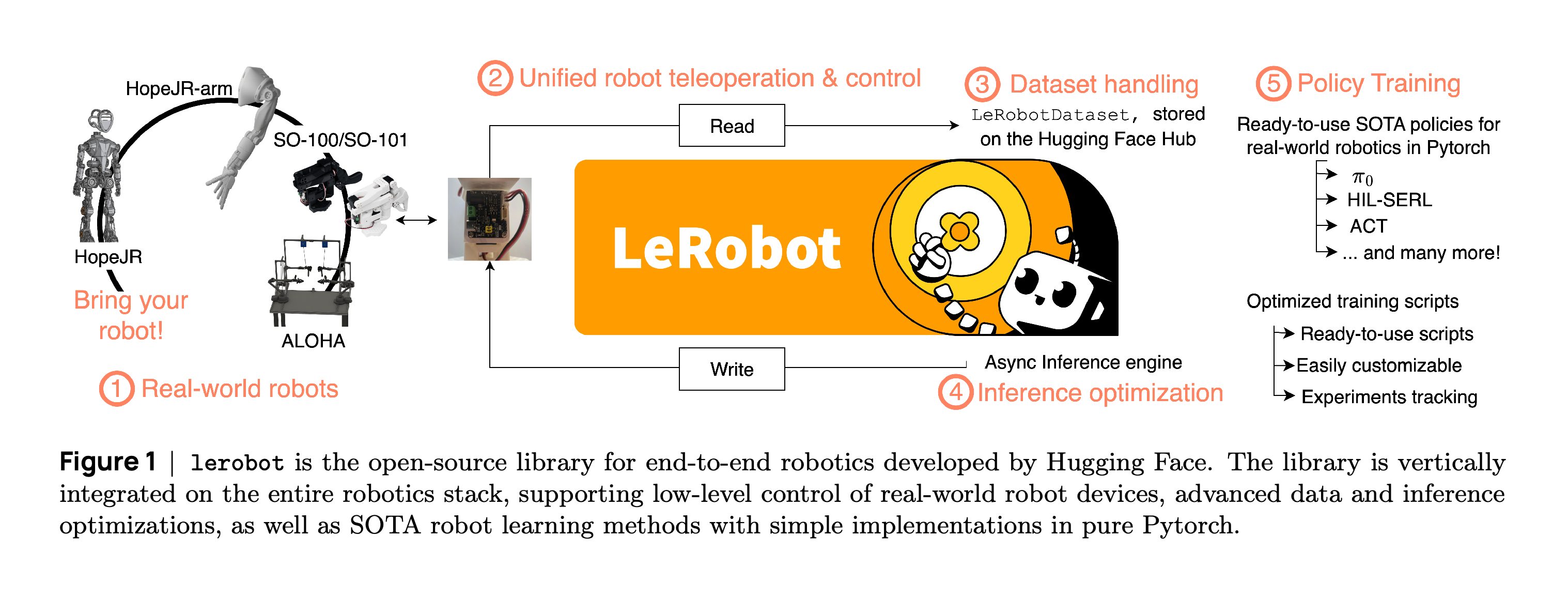
The Introduction motivates learning from data by the difficulty of accurately modeling robot-environment interactions and integrating perception, planning, and control. Figure 1 shows how lerobot connects physical robots, teleoperation, data handling, policy training, and inference optimization. The library is available at https://github.com/huggingface/lerobot.

The diagram connects hardware access, observation recording, dataset handling, policy training, and action execution in one workflow. It establishes lerobot’s coverage of the robotics stack without measuring a policy’s performance.

1.1 LeRobotDataset

LeRobotDataset provides a common interface for synchronized robot states, actions, camera streams, teleoperation status, and task descriptions. Its storage design separates the user-facing interface from tabular data, compressed video, and metadata. Multiple episodes, individual recorded task attempts, can share larger files while metadata identifies their boundaries.

• 1.1.1 The dataset class design: data/* stores frame-level Parquet tables and videos/* stores MP4 video streams. Concatenating episodes reduces file counts and filesystem pressure.
• meta/info.json records feature schemas, shapes, types, frame rate, version, and path templates; meta/stats.json supplies normalization statistics through dataset.meta.stats.
• meta/tasks.jsonl maps task descriptions to integer indices, while meta/episodes/* records episode lengths, tasks, and storage pointers.

1.2 Code Example: Batching a (Streaming) Dataset

The batching example loads lerobot/svla_so101_pickplace through LeRobotDataset or StreamingLeRobotDataset and uses delta_timestamps to request wrist-camera observations at [-0.2, -0.1, 0.0] seconds relative to a frame. Unavailable frames receive padding and a mask identifying the padded entries, and torch.utils.data.DataLoader combines samples into batches of 16. The text reports approximately 80–100 iterations per second for streaming, depending on connectivity, without a standardized hardware benchmark.

1.3 Code Example: Collecting Data

The collection example pairs an SO100Follower robot with an SO100Leader teleoperator and a 640 × 480 front camera. It specifies NUM_EPISODES = 5, FPS = 30, EPISODE_TIME_SEC = 60, and RESET_TIME_SEC = 10. The script records observations and actions, supports re-recording an episode, saves retained episodes, disconnects the devices, and calls dataset.push_to_hub().

2 Classical Robotics

Classical Robotics establishes the modeling and control concepts used to motivate learned policies, rules for selecting actions from observations. The chapter emphasizes generalization across tasks and embodiments, reduced dependence on manual modeling, and use of growing datasets. Its examples are simplified illustrations rather than experimental comparisons.

2.1 Explicit and Implicit Models

Explicit models describe robot mechanics and environmental interactions directly, whereas implicit models learn motion patterns from sensor and action data. The paper also recognizes combinations of these approaches: Temporal Difference learning, which updates value estimates using successive transitions, can complement Model-Predictive Control, which plans controls using a model, and learning can improve perception or approximate complex physical effects.

2.2 Different Types of Motion

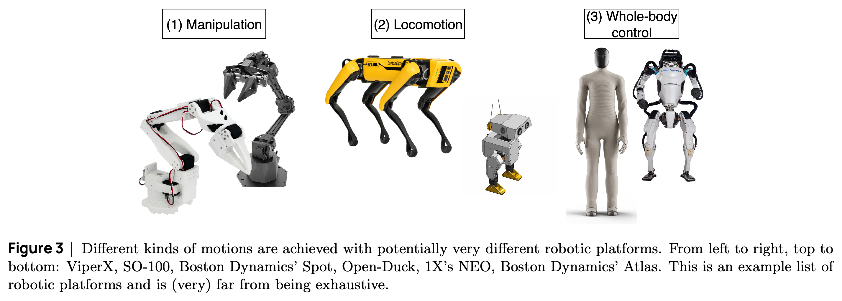
Manipulation changes the environment through actions such as grasping, locomotion changes the robot’s location, and mobile manipulation combines environmental interaction with movement. Figure 3 illustrates manipulation, locomotion, and whole-body control, coordinated motion across a robot’s body, using arms, legged robots, and humanoids. Combining movement and manipulation generally increases the number of control variables.

The robot examples clarify that changing objects, moving through an environment, and coordinating whole-body behavior involve different hardware and control requirements. The collection is illustrative and does not compare the robots’ capabilities quantitatively.

2.3 Example: Planar Manipulation

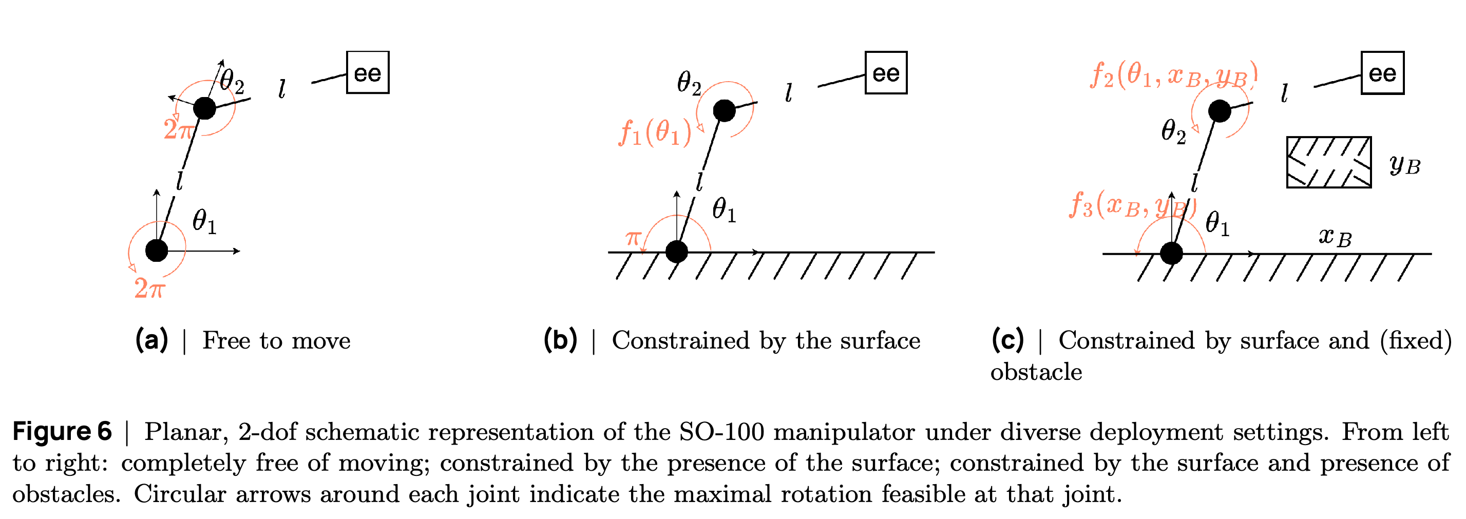
The planar manipulation example restricts the SO-100 to shoulder lift and elbow flex, leaving two motion degrees of freedom, independently controlled motion variables, plus its gripper. Forward kinematics maps joint configurations to the end-effector pose, the position and orientation of the robot’s working endpoint, while inverse kinematics finds configurations for a target pose. Surfaces and obstacles restrict feasible configurations, as Figure 6 illustrates.

• For equal link lengths l and joint angles θ₁, θ₂, the example gives p(q) = [l cos(θ₁) + l cos(θ₁ + θ₂), l sin(θ₁) + l sin(θ₁ + θ₂)]ᵀ and minimizes squared distance to the target position. This simplified model disregards endpoint orientation and initially assumes unrestricted joint rotation.
• Differential inverse kinematics solves for joint velocities through the Jacobian, the matrix relating joint changes to pose changes, and integrates those velocities to obtain successive configurations.
• 2.3.1 Adding Feedback Loops: measured pose error adjusts the velocity command to compensate for disturbances; the moving-obstacle example also motivates monitoring robot-object distance. Gain tuning remains system-specific, and intermittent contact complicates stability and tracking.

Adding a supporting surface and then an obstacle changes the allowable joint rotations of the same two-joint arm. The example shows why finding a configuration for a target position must account for environmental constraints.

2.4 Limitations of Dynamics-based Robotics

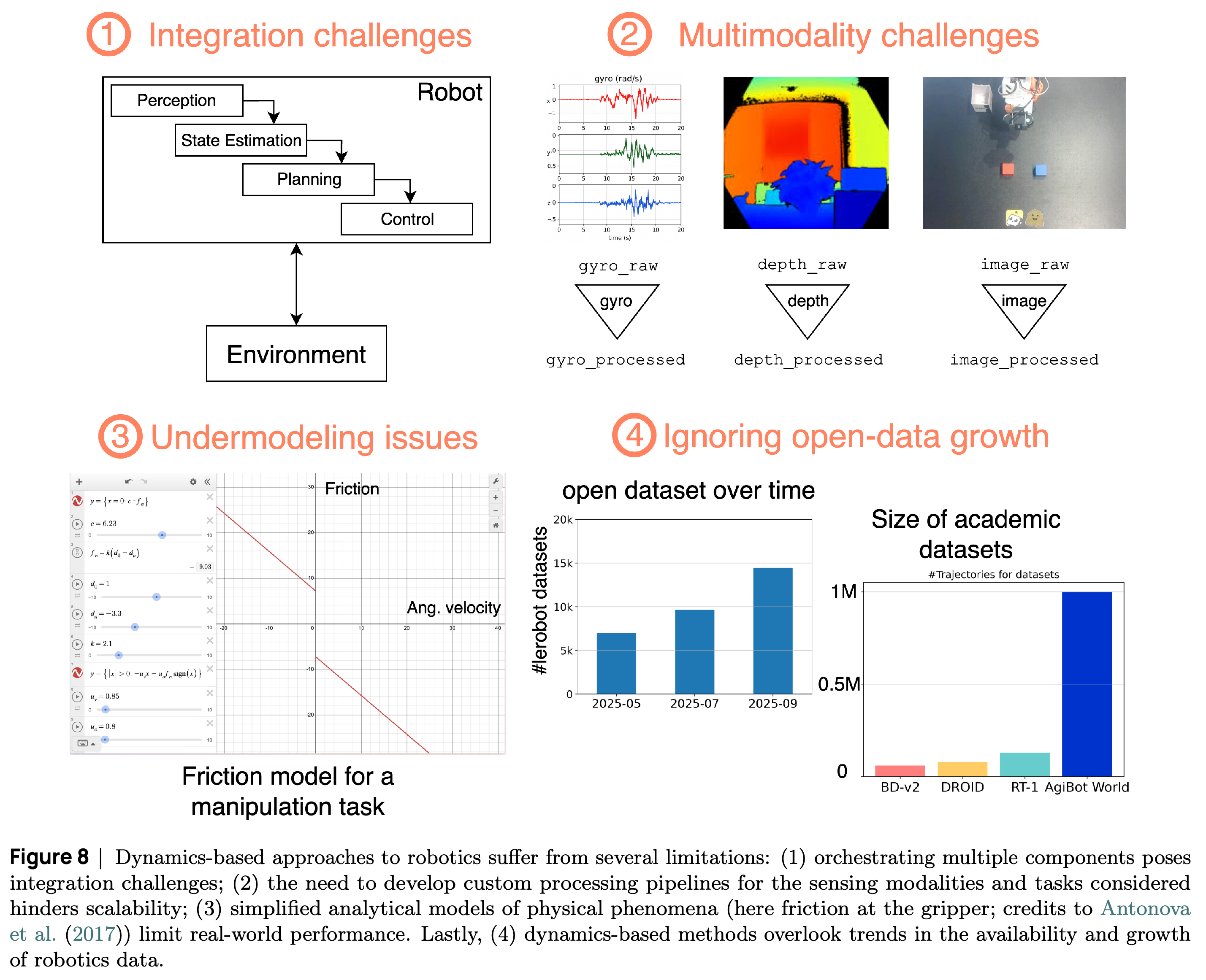
The paper identifies four limitations of dynamics-based pipelines: integration between independently engineered modules, custom processing for different sensing modalities, inaccurate physical approximations, and limited use of growing robot datasets. Figure 8 organizes these arguments. The text emphasizes accumulated interface errors, task-specific redesign, and difficulty modeling contact, friction, compliance, or deformation under force, and deformable objects.

The four panels organize the chapter’s critique into module integration, modality-specific processing, approximate physics, and limited use of data growth. The schematic and dataset plots motivate learning but do not provide a controlled comparison of classical and learned controllers.

3 Robot (Reinforcement) Learning

Learned visuomotor policies map visual and robot-state observations to actions, consolidating perception and control while learning features from heterogeneous inputs. The chapter groups methods into RL and BC, placing generalist demonstration-trained policies alongside BC because their training still largely reproduces recorded trajectories. It does not identify a universally superior approach.

3.1 A (Concise) Introduction to RL

RL represents interaction using a Markov Decision Process (MDP), a framework specifying states, actions, transition dynamics, rewards, an initial-state distribution, a discount factor, and a horizon. The tutorial primarily considers discrete-time, finite-horizon episodes and maximizes expected discounted return. State-value and state-action-value functions estimate future reward from a state or state-action pair.

• The return is \(G(\tau)=\sum_{t=0}^{T-1}\gamma^t r_t\), where \(\gamma\in[0,1)\) controls the relative weight of future rewards.
• Figure 13 distinguishes model-free methods, which learn without an explicit transition model, from model-based methods that use one. Continuous robot controls motivate policy optimization and actor-critic approaches that learn both action selection and value estimates.

3.2 Real-world RL for Robotics

Real-world RL faces unsafe exploration, slow collection of transitions, individual state-action-reward-next-state records, and repeated environment resets. Simulation improves throughput but introduces a reality gap, the mismatch between simulated and physical dynamics. Domain randomization varies simulated parameters during training, yet choosing parameters and distributions remains difficult and cannot resolve every fidelity limitation.

• Soft Actor-Critic (SAC), an off-policy actor-critic method that can learn from previously collected actions and rewards while encouraging diverse actions, reuses transitions through a replay buffer, a store of past experience. Reinforcement Learning with Prior Data (RLPD) samples offline and online transitions in equal proportions without a separate pretraining stage.
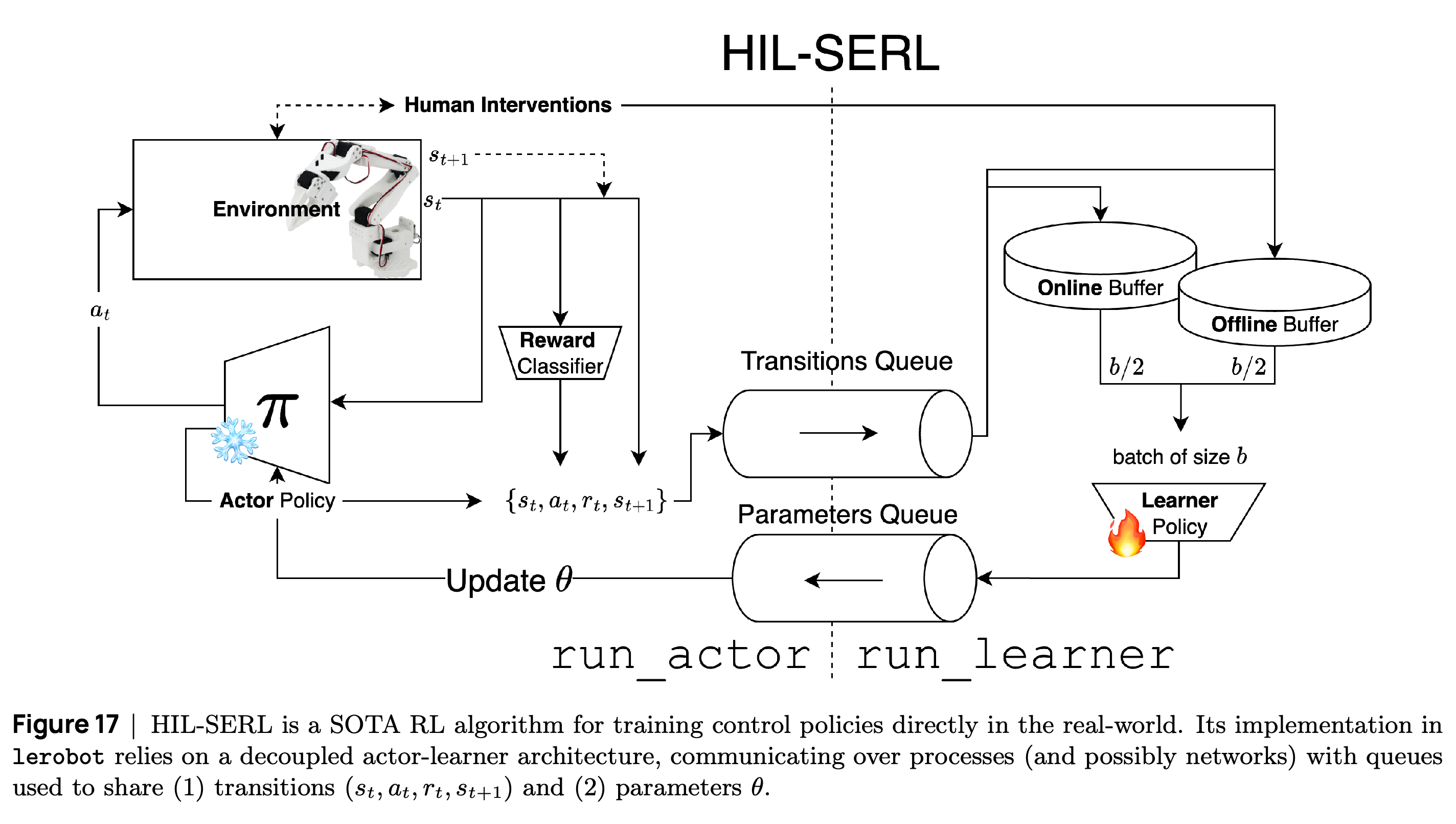
• SERL, a software suite for sample-efficient robotic RL, adds learned success classifiers and forward/backward controllers for task execution and resetting. HIL-SERL inserts targeted human corrections into both replay buffers, increasing their sampling frequency; the tutorial attributes 99%+ success within 1–2 hours to Luo et al. (2024).
• 3.2.1 Code Example: Real-world RL trains a reward classifier, defines an actor for hardware interaction and a learner for parameter updates, and connects them through transition and parameter queues, as Figure 17 shows. 3.2.2 Limitations of RL in Real-World Robotics: Simulators and Reward Design emphasizes expensive experience collection, difficult contact simulation, and reward shaping, the addition of intermediate reward signals, that can encourage unintended solutions.

Transitions flow from the actor to the learner, while updated policy parameters flow back. Equal sampling from online and offline buffers, together with insertion of human interventions into both buffers, explains how corrections receive repeated training exposure while hardware interaction and optimization run separately.

4 Robot (Imitation) Learning

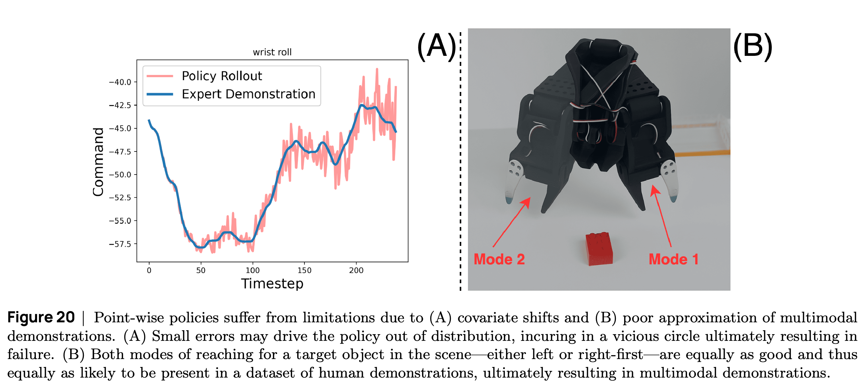
BC learns observation-to-action behavior from offline expert trajectories without requiring rewards or online exploration during training. The paper identifies sequentially dependent samples, covariate shift, deployment observations departing from the training distribution, and multimodal demonstrations, several valid action strategies for similar observations, as central difficulties. Offline training avoids training-time exploration on hardware but does not establish safe deployment.

• Figures 18 and 19 use lerobot/svla_so101_pickplace to illustrate synchronized joint measurements, images, and expert actions; Figure 18 summarizes the first 5 recorded episodes with means and standard deviations.
• Figure 20 explains how prediction errors can accumulate and how a point-estimate policy, which outputs one action prediction, can average incompatible valid strategies. The tutorial also warns that imitation inherits demonstration quality and may lack recovery behavior absent from the data.

The trajectory panel illustrates divergence between expert commands and policy execution, while the grasping panel shows two valid approaches to the same object. Together they distinguish accumulated execution errors from the difficulty of representing multiple valid action modes.

4.1 A (Concise) Introduction to Generative Models

Generative models learn distributions over demonstrations so that a policy can represent multiple plausible behaviors. This section develops latent-variable models, which introduce unobserved factors influencing the data, followed by diffusion and flow matching as foundations for action-generating policies.

• 4.1.1 Variational Auto-Encoders: a variational auto-encoder (VAE) learns a decoder and an approximate posterior, a distribution over latent factors inferred from observed data. The Evidence Lower Bound (ELBO), a tractable lower bound on log-likelihood, combines reconstruction with Kullback–Leibler divergence, a distribution discrepancy that regularizes the posterior toward a prior, the latent distribution specified before observing a sample.
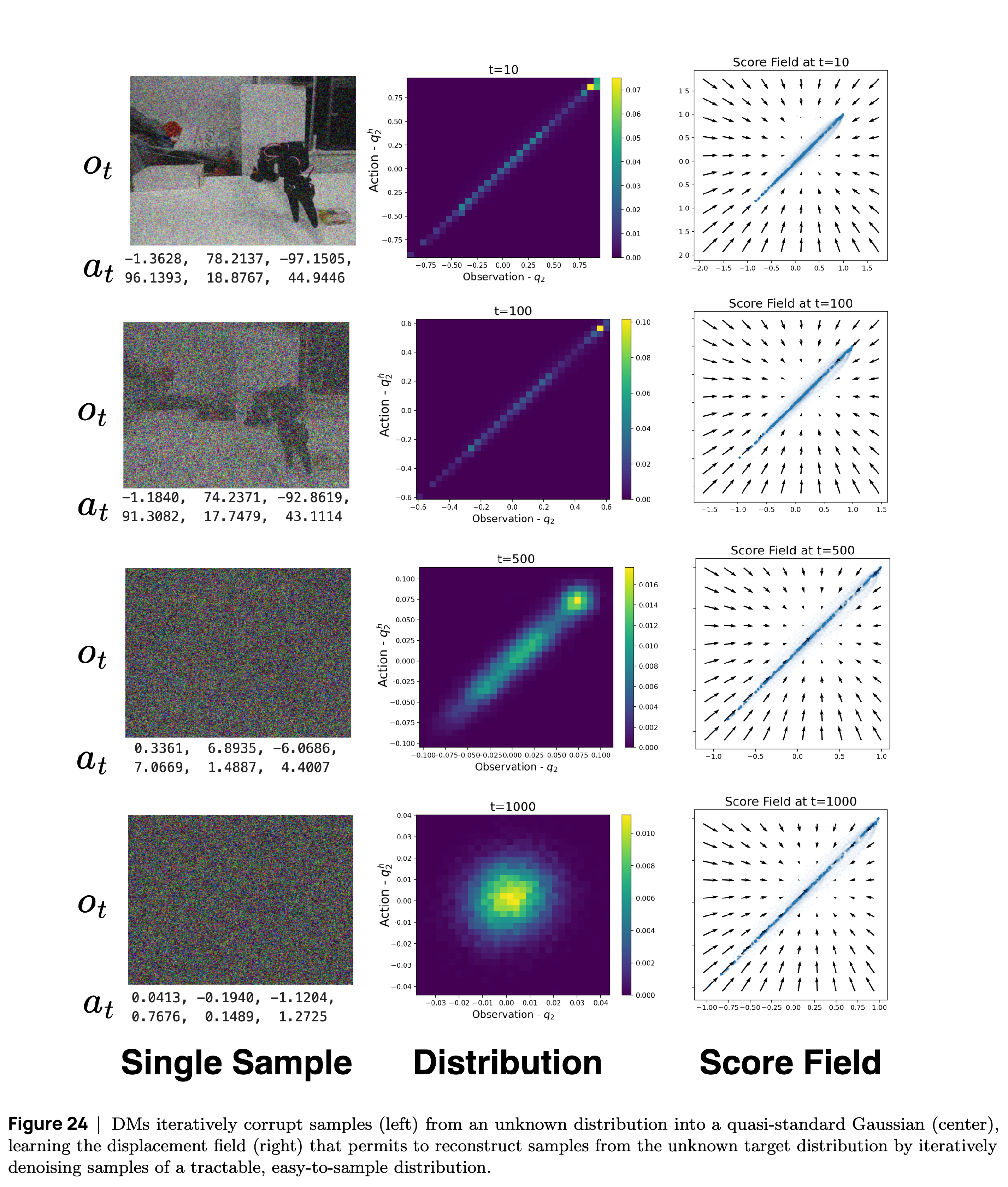
• 4.1.2 Diffusion Models: training progressively corrupts data with Gaussian noise and learns to reverse the corruption. Figure 24 illustrates this process for robot observation-action samples, while the simplified objective trains a noise predictor at a randomly selected diffusion step.
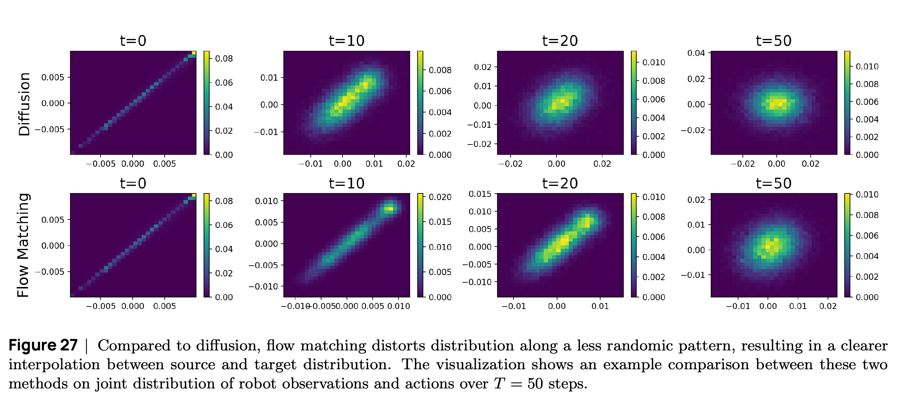
• 4.1.3 Flow Matching: training fits a vector field, a rule assigning an instantaneous direction and speed to each sample, that transports samples from a simple prior to the data distribution. Conditional flow matching uses \(z_t=(1-t)z_0+t z_1\) and target velocity \(z_1-z_0\); inference numerically integrates the learned field, and Figure 27 compares illustrative distribution paths over \(T=50\) steps.

Successive rows show increasingly corrupted observations and actions, changes in their distribution, and fields associated with reconstruction. The illustration explains diffusion’s learning problem through robot data without reporting downstream control accuracy.

The two rows compare diffusion and flow-matching transformations at selected steps over T = 50. The flow-matching row retains a more structured intermediate distribution, illustrating the discussion of more direct probability paths; the figure does not measure inference speed or robot task success.

4.2 Action Chunking with Transformers

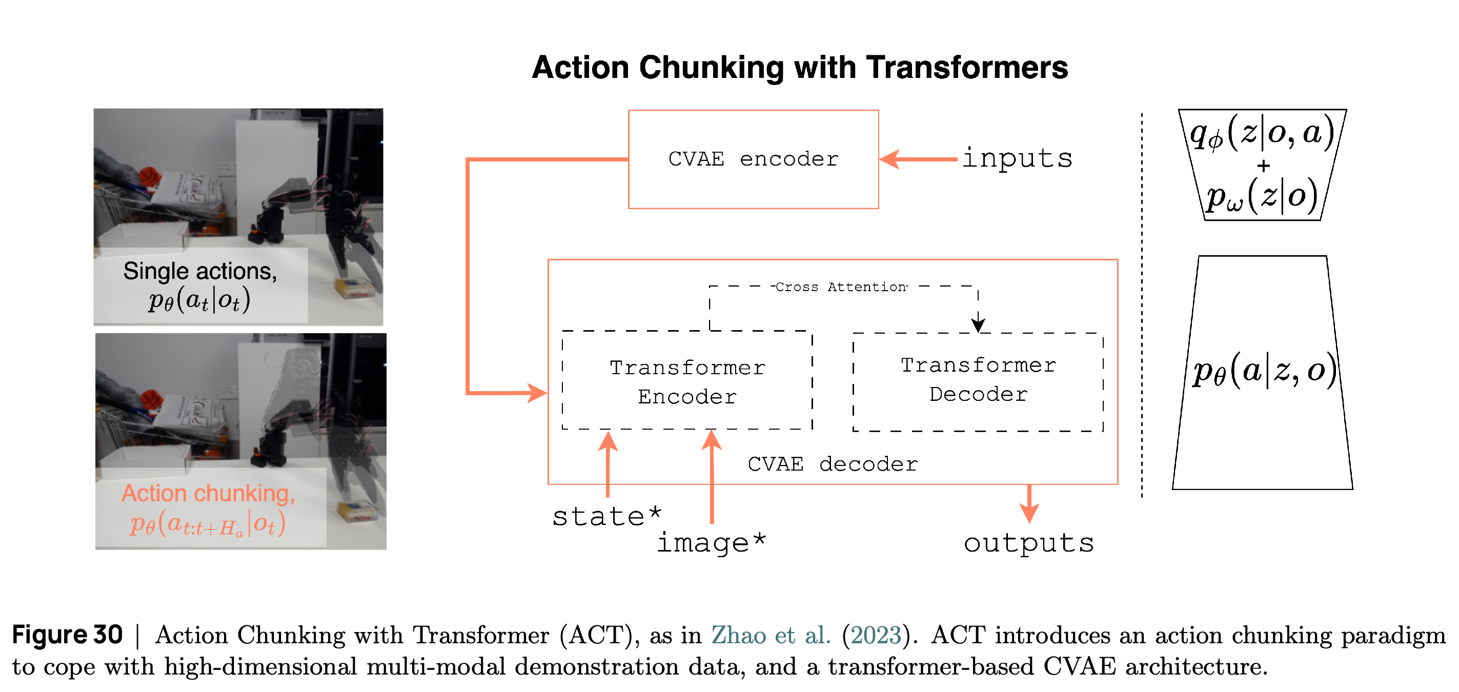
Action Chunking with Transformers (ACT) combines a transformer, an attention-based sequence architecture, with a Conditional VAE, a latent-variable generator conditioned on observations, to predict several future actions together. The tutorial reports Zhao et al. (2023)’s ablations of 1% versus 44% success without versus with chunking, and a −33.3% performance change when replacing the variational objective with standard supervised learning on human demonstrations. The objectives performed comparably on scripted demonstrations; the tutorial does not specify whether −33.3% denotes a relative change or percentage points.

• The encoder summarizes action chunks and robot-state information into a style variable during training. At test time, the encoder is discarded and \(z=0\) is used, while the decoder receives images and robot-state observations, as Figures 28–30 explain.
• Overlapping action chunks can be combined using an exponential moving average, a weighted aggregation across predictions, to reduce open-loop execution, acting without incorporating a new observation.
• 4.2.1 Code Example: Training and Using ACT in Practice uses ACTConfig, ACTPolicy, dataset-derived features, normalization, and delta_timestamps on lerobot/svla_so101_pickplace. The printed training example sets batch_size = 32 and training_steps = 1, demonstrating the workflow without reproducing the cited success rates; deployment requires camera names and resolutions to match training.

The diagram links ACT’s training-only latent encoder to its observation-conditioned transformer decoder and contrasts a single action with an action sequence. It explains the architecture behind the cited chunking ablation; the numerical success comparison appears in the surrounding text.

4.3 Diffusion Policy

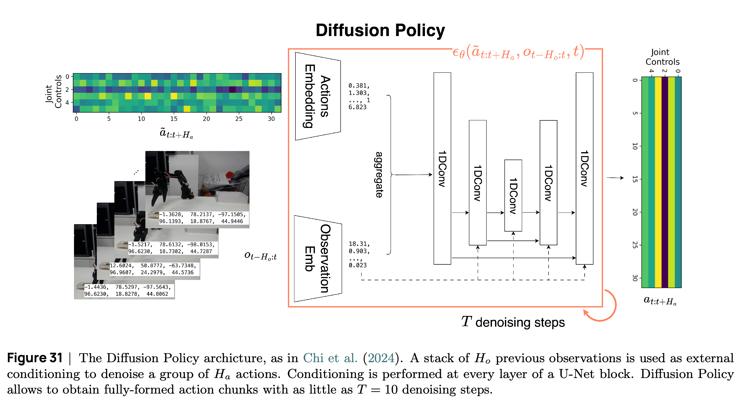
Diffusion Policy conditions an action-chunk noise predictor on a history of images and robot-state observations, generating actions while keeping the observations fixed. The tutorial reports training with 50–150 demonstrations, approximately 15–60 minutes of teleoperation. It attributes visual-policy success comparable to state-based policies using privileged information, simulator state unavailable to a deployed robot, to the cited evaluations.

• Figure 31 shows the convolution-based U-Net, an encoder-decoder network with connections between corresponding intermediate layers, conditioning denoising on observations throughout the network. Action chunks can be generated with as few as \(T=10\) denoising steps.
• Denoising Diffusion Implicit Models provide the deterministic sampling variant described here, with 10x fewer denoising steps than the referenced probabilistic variant. Transformer predictors can perform strongly but are more sensitive to hyperparameters; the tutorial recommends convolution-based predictors as a starting point while noting a bias toward low-frequency, slowly varying action components.
• 4.3.1 Code Example: Training and Using Diffusion Policies in Practice uses DiffusionConfig and DiffusionPolicy with observation and action windows. Its batch_size = 32 and training_steps = 1 are illustrative settings; the deployment example loads a checkpoint, applies preprocessing and postprocessing, and sends actions to the robot.

A noisy action sequence and a history of observations enter the conditional denoising network, which repeatedly refines the sequence. Conditioning within the network explains how Diffusion Policy generates future actions while keeping observed images and states fixed.

4.4 Optimized Inference

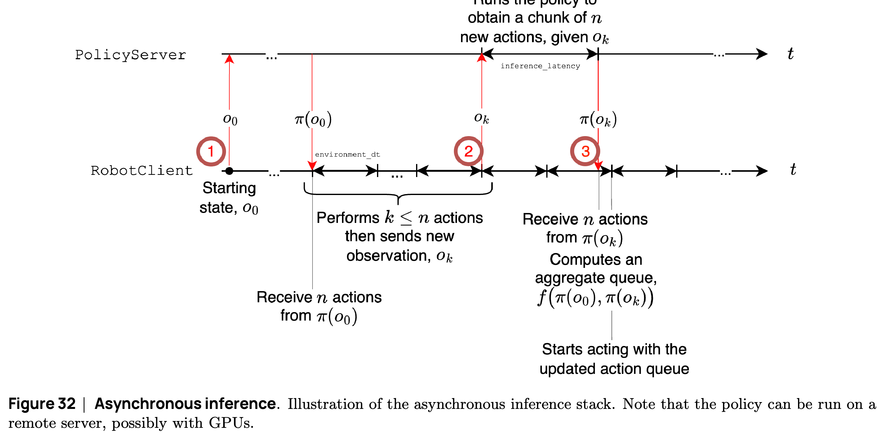
Optimized Inference separates action-chunk prediction from execution so that RobotClient can consume queued actions while PolicyServer computes replacements, potentially on another machine. Figures 32 and 33 explain the trade-off between prediction frequency, computational cost, and an empty action queue. Avoiding pauses requires replacement chunks to arrive before the available actions are exhausted.

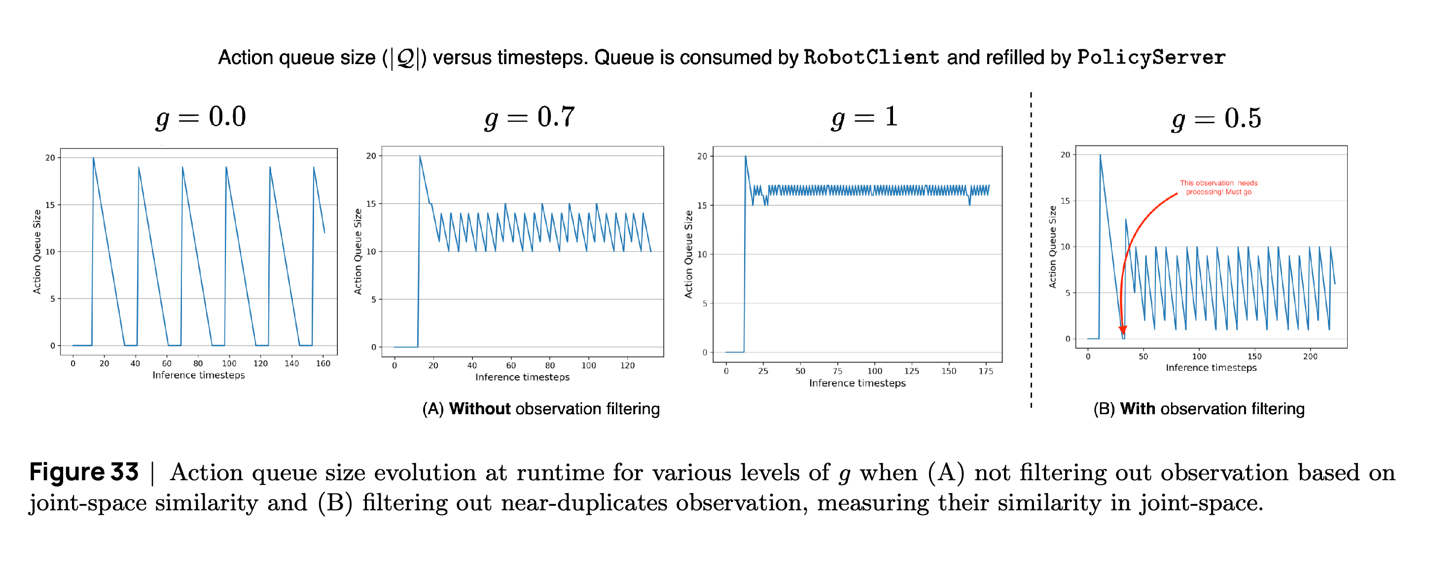
• New inference is triggered when |Aₜ|/Hₐ < g, where Hₐ is the chunk size and \(g\in[0,1]\) is the queue threshold. Near-duplicate observations are filtered by joint-space distance, the distance between joint configurations, but an empty queue forces processing of the latest observation.
• At 30 frames per second, the paper uses \(\Delta t=33\,\mathrm{ms}\) and gives g ≥ E[ℓₛ]/(HₐΔt) as an average-latency condition for avoiding queue exhaustion, assuming communication time is negligible relative to server inference latency ℓₛ. Because this uses expected latency, it does not guarantee that the queue remains nonempty under latency variation.
• 4.4.1 Code Example: Using Async Inference configures PolicyServerConfig and RobotClientConfig with policy_type=”smolvla”, pretrained_name_or_path=”fracapuano/smolvla_async”, chunk_size_threshold=0.5, and actions_per_chunk=50, then runs an action-receiver thread alongside the control loop. Camera specifications must match the policy, and actions_per_chunk must remain below its maximum supported action count.

The timeline shows the client executing available actions during server inference and combining a returned chunk with remaining queued actions. This overlap illustrates how prediction can begin before the current sequence ends and how a separate policy server can support the control loop.

The traces compare g = 0.0, g = 0.7, and g = 1 without observation filtering, then g = 0.5 with filtering. They illustrate empty-queue pauses, earlier replenishment, and forced processing of a similar observation when the queue empties.

5 Generalist Robot Policies

Generalist Robot Policies extends the discussion from individual tasks to policies trained across tasks, environments, and embodiments. Its organizing principle is pretraining on broader data followed by task adaptation, supported by pretrained perception models, expressive action generators, and aggregated demonstration datasets.

5.1 Preliminaries: Models and Data

Robot data is expensive to collect and tied to hardware and operating conditions, so aggregation must handle heterogeneous state and action representations and possible negative transfer, where combining data harms performance. The tutorial traces development from BC-Zero, a demonstration-trained latent-variable policy, through Robotics Transformer 1 (RT-1) and RT-2 to open VLA models. It describes RT-1 training on 130k trajectories collected over 13 robots and 17 months, and RT-2 combining web and robot data to reuse visual-semantic knowledge.

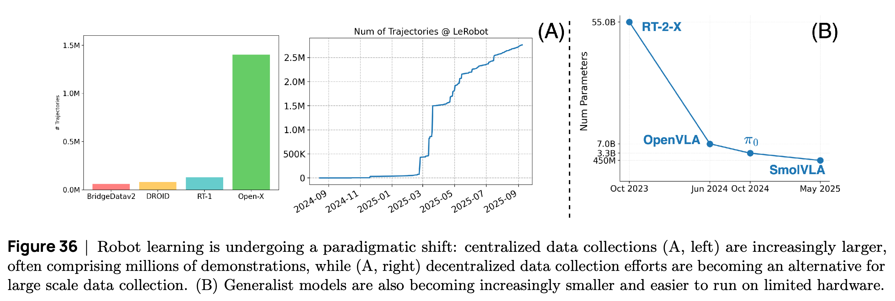
• Open X-Embodiment aggregates 60 datasets from 22 robot embodiments and 21 institutions into 1.4M trajectories. The cited work reports that a model trained across embodiments can outperform specialist models trained on their respective single-embodiment datasets.
• The Distributed Robot Interaction Dataset (DROID) contains 75k+ human demonstrations in realistic manipulation settings. OpenVLA uses 970k+ Open-X trajectories, shares weights and training recipes, and predicts discrete action tokens, categorical representations of controls, with 256 levels.
• Figure 36 contrasts increasing centralized and community data collections with decreasing parameter counts of selected models. These examples support the accessibility discussion but do not isolate how parameter count affects deployment performance.

The data panels compare centralized trajectory collections with community collection over time, while the model panel shows decreasing parameter counts for selected models. The figure supports the historical accessibility discussion without measuring matched task performance or runtime costs.

5.2 VLAs

Modern VLAs discussed here combine a Vision-Language Model (VLM), a model that processes images and text together, with an action expert, a specialized component that predicts continuous action chunks. The tutorial describes separate parameter sets within a unified transformer as a Mixture of Experts architecture, allocating distinct weights to visual-semantic processing and robot control. This description concerns π₀ and SmolVLA; earlier models in the tutorial predict discrete actions.

• 5.2.1 VLMs for VLAs explains how pretrained vision encoders, which map images to features, and large language models, text models trained at scale, are combined and trained on image-text data before supervised instruction fine-tuning.
• The proposed benefit is reuse of visual and semantic representations for interpreting robot instructions and recognizing objects. The text presents generalization to novel scenarios as a possibility and emphasizes efficient computation for deployment.

5.3 π₀

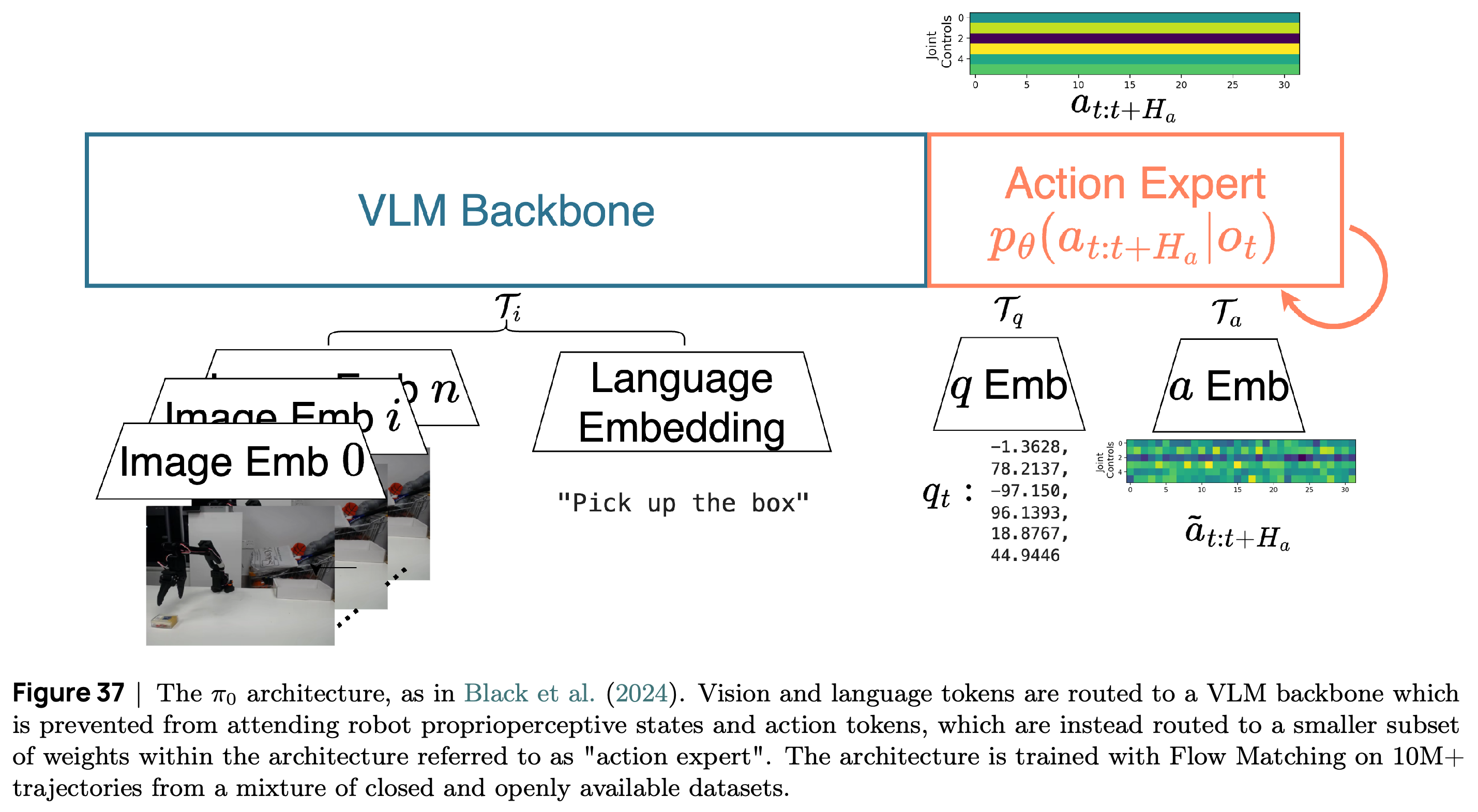
π₀ combines a PaliGemma vision-language backbone with a 300M-parameter action expert that generates continuous action chunks through flow matching. Figure 37 shows separate image-language, robot-state, and action-token blocks. Blockwise causal masking, allowing attention within each block while blocking access to later blocks, prevents image-language tokens from attending to robot-state and action tokens and enables reuse of cached attention information during iterative generation.

• The π dataset contains 10M+ trajectories, with approximately 9.1% openly available; its demonstrations span 7 robot configurations and 68 tasks. The tutorial reports that pretraining followed by fine-tuning consistently outperforms a task-specific π₀ model trained from scratch in the cited benchmarks, while much of the pretraining data remains undisclosed.
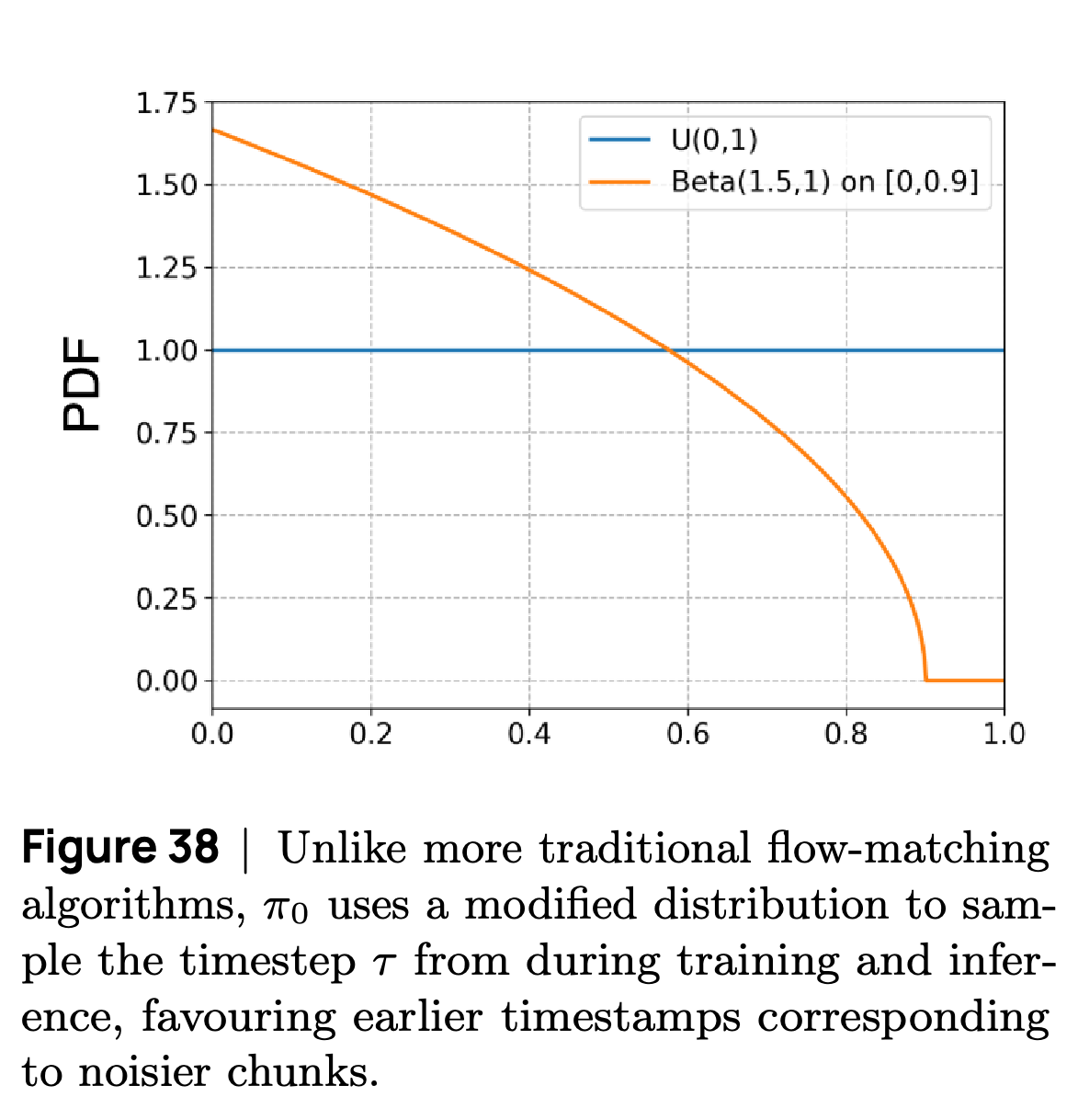
• Inference can use as few as 10 flow-integration steps. Figure 38 illustrates modified training-time timestep sampling intended to emphasize noisier action chunks; the text also cites later evidence that allowing action-training gradients to modify the vision-language backbone can harm performance.
• 5.3.1 Code Example: Using π₀ loads lerobot/pi0_base through PI0Policy, supplies a task description and robot_type, and configures three camera slots. The model handles robots with fewer motion variables through zero-padding and fewer camera views through masked slots; deployment camera specifications must match the policy.

Images and instructions enter the vision-language backbone, while robot state and noisy actions enter the action expert. The separation and attention restrictions explain specialization and why image-language attention information can be cached across action-refinement steps.

The plotted density contrasts uniform sampling with the modified timestep sampling described for π₀. It illustrates the intended emphasis on noisier action chunks; the tutorial’s stated Beta(1.5,1) distribution and the decreasing plotted curve do not provide an unambiguous mathematical specification.

5.4 SmolVLA

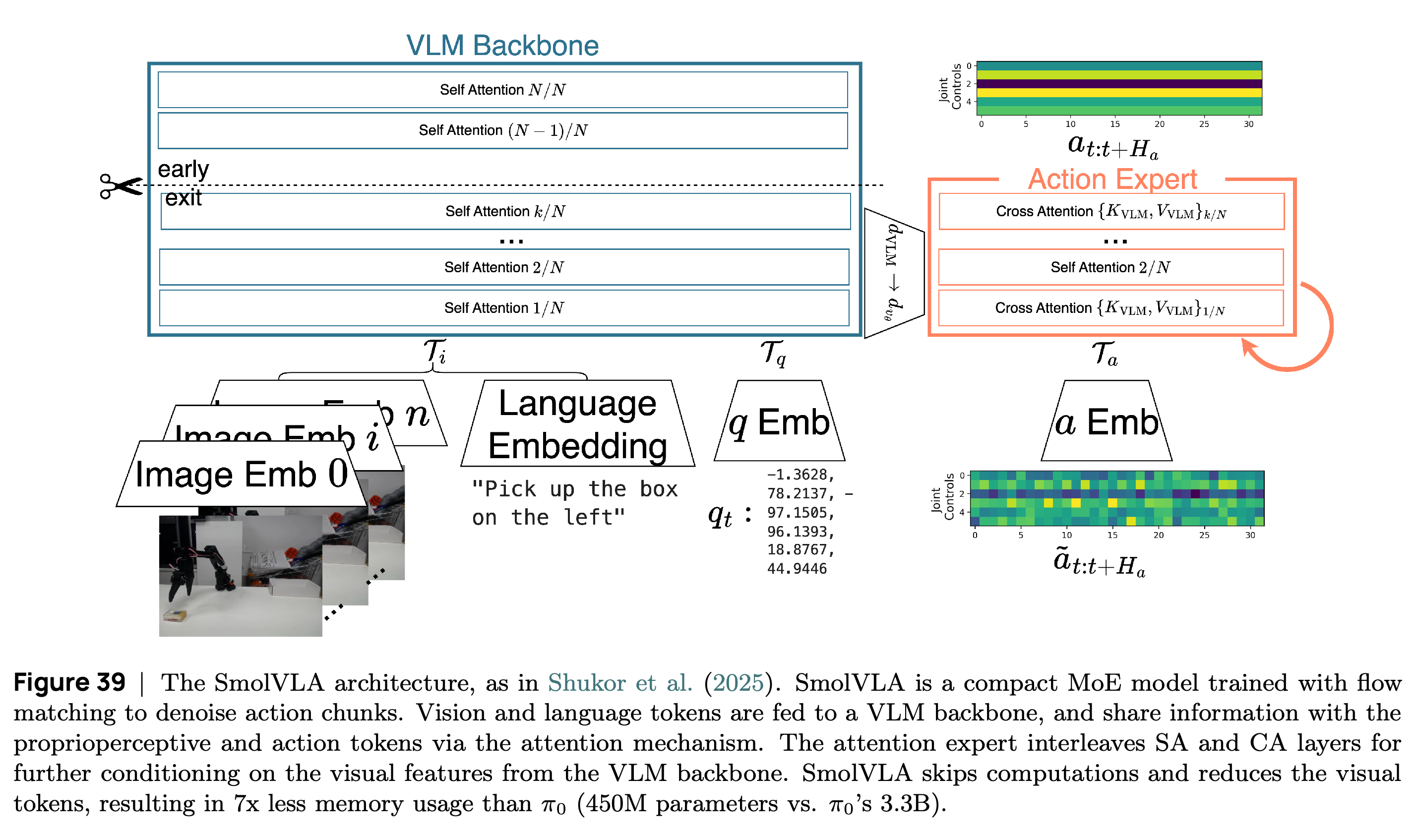
SmolVLA uses the compact SmolVLM-2 vision-language backbone and an approximately 100M-parameter action expert, totaling approximately 450M parameters versus π₀’s 3.3B. Its pretraining uses 450+ community datasets totaling 20k+ trajectories. Task re-annotation and a standardized top/wrist/side camera ordering address inconsistent community data.

• Figure 39 shows alternating self-attention, interaction among action tokens, and cross-attention, action tokens querying visual, language, and robot-state features. Compute reductions include 64 visual tokens per frame, using only the first half of the backbone’s decoder layers, and an action-expert embedding dimension of 0.75 times the backbone dimension.
• At inference, SmolVLA integrates flow over 10 steps and can separate prediction from execution. The body reports close to 40% faster operation and 6x less memory than π₀, whereas Figure 39’s caption states 7x less memory; the tutorial does not supply enough measurement detail to reconcile these ratios or generalize them across hardware.
• 5.4.1 Code Example: Using SmolVLA loads lerobot/smolvla_base with SmolVLAPolicy, prepares robot features and task text, and configures two 640 × 480 cameras at 30 frames per second. Its 5 episodes with 20 steps each illustrate deployment calls, with camera names and resolutions required to match training.

The early-exit marker and action-expert attention stack show the architectural reductions in computation described for SmolVLA. The caption reports 7x less memory than π₀, whereas the section body reports 6x less memory, leaving the comparison unresolved within the tutorial.

6 Conclusions

The Conclusions section connects classical modeling limitations, real-world RL, demonstration-based generative policies, and language-conditioned generalist models. The authors identify open datasets, accessible hardware, standardized architectures, and lerobot as enabling infrastructure. This is a synthesis of reviewed work, without a new experiment isolating the effect of openness.

Appendix

• The supplied PDF contains no separate appendix: References begins on page 67 and continues through page 76. Practical resources identified in the paper include https://github.com/huggingface/lerobot and https://github.com/fracapuano/robot-learning-tutorial. The document is arXiv:2510.12403v1, and its title page gives October 15, 2025.

Brief Thoughts

The tutorial links control concepts to dataset interfaces, training loops, and deployment scheduling, making it useful for engineers preparing a robot-learning workflow. Its quantitative claims need attribution to the cited studies: the one-step training snippets do not reproduce the reported performance, and the cross-method discussion lacks a shared evaluation protocol. The conflicting SmolVLA memory ratios also require checking the original study before using them for resource planning.