Tensor Logic: The Language of AI | Summary

Contents

Summary
1. Introduction
2. Background
- 2.1 Logic Programming
- 2.2 Tensor Algebra
3. Tensor Logic
4. Implementing AI Paradigms
5. Reasoning in Embedding Space
6. Scaling Up
7. Discussion
Appendix
Brief Thoughts

This article explains the key points of Tensor Logic: The Language of AI.

2025-10-14 (arXiv)
Domingos, Pedro.
Paul G. Allen School of Computer Science & Engineering, University of Washington
Paper
Project Page

Summary

Tensor Logic: The Language of AI addresses the separation between neural computation, which learns numerical representations from data, and symbolic reasoning, which derives conclusions from explicit rules and facts. Its central result is a shared formulation using tensor equations, equations over indexed multidimensional arrays, compared conceptually with the separate capabilities of Python-based learning libraries and logic programming languages; the paper reports no benchmark comparison.
The construction represents relations as sparse Boolean tensors, arrays that store true or false values with mostly false entries, and Datalog rules, rules in a fact-and-rule logic programming language, as Einstein summation followed by thresholding. Einstein summation combines indexed tensor products with summation over selected indices, while thresholding converts positive counts of supporting facts into truth values.
The paper gives equation-based implementations of neural networks, symbolic systems, kernel machines, predictors based on pairwise similarity functions, and probabilistic graphical models, distributions represented by interacting factors. It also proposes reasoning in embedding space, where objects and relations have numerical representations, and two scaling strategies. The evidence consists of mathematical constructions and implementation proposals, without reported training runs, accuracy results, hardware measurements, or measured speedups.

1. Introduction

The introduction argues that an AI programming language should integrate prior knowledge, automated reasoning, learning, transparency, reliability, and scalability. The author describes LISP and Prolog, languages used for symbolic AI, as limited in learning and scalability, and Python with PyTorch or TensorFlow, numerical learning libraries, as lacking native reasoning and knowledge acquisition. Tensor logic proposes to unify the mathematical foundations of these capabilities.

2. Background

The background develops the correspondence between logic programming and tensor algebra. Logic programming supplies facts, rules, and procedures for deriving answers; tensor algebra supplies indexed arrays and operations that can express those procedures numerically.

2.1 Logic Programming

A Datalog program consists of facts and rules. A rule joins relations by matching shared arguments, then projects the result by discarding arguments absent from its head, the conclusion: Ancestor(x,z) ← Ancestor(x,y),Parent(y,z) matches on y and retains x and z. With Ancestor(Alice,Bob) and Parent(Bob,Charlie), this derives Ancestor(Alice,Charlie).

Forward chaining repeatedly applies rules until no additional facts follow; the resulting set is the deductive closure or fixpoint. Backward chaining starts from a query and recursively seeks supporting facts or rules.
Both procedures are sound for Datalog: their answers follow logically from the supplied rules and facts. A rule has declarative semantics as a statement about the world and procedural semantics as a computation of its head from its body, the supporting conditions.
Inductive logic programming (ILP), learning logic programs from data, can induce rules and perform predicate invention, discovering relations absent from the original data.

2.2 Tensor Algebra

A tensor has an element type and a shape specifying the size along each index; its rank is its number of indices. Einstein notation expresses matrix multiplication as \(C_{ik}=\sum_j A_{ij}B_{jk}\), summing over the shared index j. Tucker decomposition represents a tensor using a smaller core tensor and factor matrices that map the core’s indices to the original dimensions.

The rank-3 example is \(A_{ijk}=M_{ip}M’_{jq}M’‘_{kr}C_{pqr}\), where C is the core and M, M′, and M″ are factor matrices. This representation later connects compression, learning, and embedded relations.

3. Tensor Logic

Tensor logic uses tensor equations as its sole program construct. The following subsections define the representation, execution procedures, and learning mechanism around the correspondence between relations and Boolean tensors and between logical rules and tensor operations.

3.1 Representation

For Aunt(x,z) ← Sister(x,y),Parent(y,z), the corresponding equation is \(A_{xz}=H\left(\sum_y S_{xy}P_{yz}\right)\), where H(x) = 1 if x > 0 and 0 otherwise. Multiplication matches compatible facts, summation removes y, and the step function converts any positive number of supporting matches into Boolean truth.

Tensor projection sums over removed indices. Tensor join multiplies entries with matching values of common indices while retaining those indices; join followed by projection performs the summation. With no common indices, join becomes a tensor product; with all indices shared, it becomes an elementwise product.
An equation’s right-hand side contains joins, projection onto its left-hand-side indices, and an optional elementwise nonlinearity. Only indices absent from the left-hand side are summed out: Y = step(W[i] X[i]) computes a thresholded dot product, whereas Y[i] = step(W[i] X[i]) retains i.
Entries default to 0, and equations with the same left-hand side are implicitly summed. Parentheses denote Boolean tensors and permit Datalog facts; square brackets denote indexed tensors. File assignment reads or writes tensors, and proposed notation conveniences include index functions, normalization, alternative projection operators, slices, and external functions.
X[i,j] = sig(W[i,j,k] X[i−1,k]) describes a multilayer perceptron (MLP), a network of successive weighted layers, with sig denoting the sigmoid function, a smooth mapping to values between 0 and 1. The recursive neural network (RNN) example updates a state over time using a virtual index that reuses storage; the author invokes the cited network’s Turing completeness, its ability to express general computation, to argue the same for tensor logic.

3.2 Inference

Forward chaining executes equations in turn whenever their inputs are available, repeating until no new elements can be computed or a stopping criterion is met. Backward chaining treats equations as functions: a query recursively requests the tensors needed for its answer, with elements assigned 0 when neither data nor an equation supports them. The execution direction depends on the application.

3.3 Learning

The learning construction expresses gradients, derivatives used to update parameters, as another tensor logic program. For a product equation with a factor appearing once, differentiating with respect to that factor leaves the product of the other factors; the loss gradient also incorporates the nonlinearity’s derivative and contributions from equations using that tensor. Training requires equations defining the loss, and tensors not supplied as training data are learned by default unless designated constant.

The illustrative squared loss is Loss = (Y[e] − X[*e,N,j])², with e indexing examples, N identifying the final layer, and j indexing units. The virtual example index permits storage reuse, and the optimizer may be supplied externally or expressed in tensor logic.
Backpropagation through structure, computing parameter updates along each example’s derivation, accommodates different equations being used by different examples. Backpropagation through time is its special case for the recursive network.
Learning a Tucker decomposition from a supplied data tensor produces a core and factor matrices; thresholding them into Boolean values yields invented predicates. The paper presents this connection without evaluating the resulting predicates.

4. Implementing AI Paradigms

The implementations use forward chaining unless otherwise specified. The section expresses four established AI paradigms through tensor equations, with operational explanations of how their components map to the notation.

4.1 Neural Networks

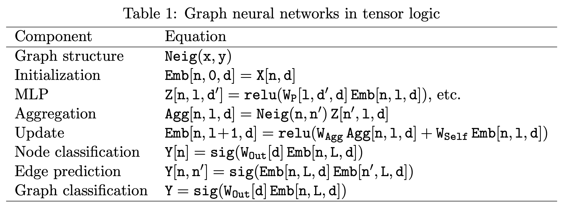
Convolution applies a shared filter across image positions, and pooling combines nearby outputs. Pooled[x/S,y/S] = Features[x,y] uses integer division and stride S, the size of each pooling block, to implement sum-pooling; max= substitutes maximum aggregation. Table 1 expresses a graph neural network (GNN), a neural network operating on graph-structured data, through node transformations, neighbor aggregation, and embedding updates.

The Boolean relation Neig(n,n′) selects adjacent nodes. Joining it with transformed features and summing out n′ aggregates neighbors; node-independent transformation weights preserve the computation under node relabeling.
Each layer performs message passing, combining neighboring nodes’ information to update node representations. The table supplies final output equations for node classification, edge prediction, and graph classification.

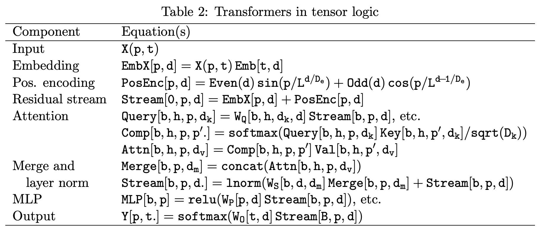
Attention weights value vectors according to comparisons between query and key vectors, learned projections of the inputs. Table 2 extends this construction to a transformer, an attention-based neural architecture, using token embeddings, positional encoding to represent sequence positions, a residual stream carrying intermediate representations, multiple attention heads, normalization, and output token probabilities. The author describes an entire transformer using just a dozen tensor equations, although some components are abbreviated with “etc.” or left unshown.

The attention comparison uses softmax, normalization into positive weights summing to 1, over the key-position index. Comparisons are scaled by sqrt(D_k), the square root of the key dimension, before the weighted value sum removes that position index.
Block and head indices organize repeated attention computations. Head outputs are concatenated, combined with the residual stream, and layer-normalized, rescaled across feature dimensions; subsequent MLP processing is partly omitted from the table.

4.2 Symbolic AI

Every Datalog program is a valid tensor logic program, supporting Datalog-style reasoning and planning in function-free domains, where expressions contain no function terms. Supporting functions as in Prolog additionally requires unification, finding substitutions that make expressions match. The paper identifies this requirement without presenting a complete Prolog implementation.

4.3 Kernel Machines

A kernel machine is written as Y[Q] = f(A[i] Y[i] K[Q,i] + B), where Q is the query example, i ranges over support vectors, examples contributing to the prediction, A supplies coefficients, B is a bias, and f is an output nonlinearity. Separate equations define polynomial and Gaussian kernels; K is their Gram matrix, the matrix of pairwise kernel values between examples. Structured prediction, producing interrelated output elements, uses vector outputs and equations describing interactions among outputs and between outputs and inputs.

4.4 Probabilistic Graphical Models

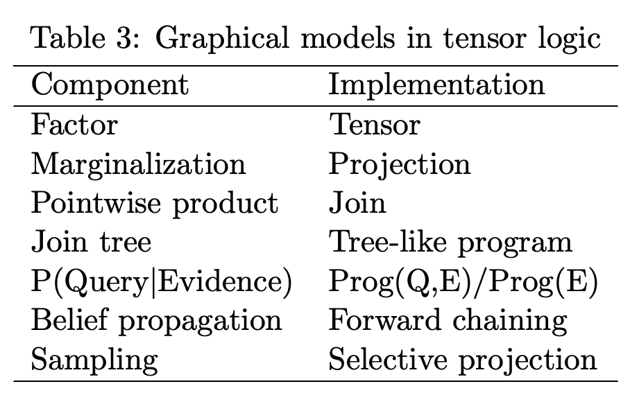
A discrete probabilistic graphical model represents a joint distribution as a normalized product of nonnegative factors, functions over subsets of variables. Table 3 maps factors to tensors, marginalization, summing out variables, to projection, and pointwise factor multiplication to join. A join tree, a tree of combined factors used for inference, becomes a tree-like tensor logic program evaluated by backward chaining.

For a Bayesian network, whose factors are conditional distributions given parent variables, the normalization constant is 1. Evidence is supplied as facts; ratios of program evaluations yield evidence and conditional probabilities, as summarized in Table 3.
The stated linear-time inference condition is linearity in the size of the join tree. This tree can be exponentially larger than the original model, so the construction retains the underlying inference complexity.
For approximate inference, loopy belief propagation, iterative updates of probabilistic information, maps to forward chaining. Monte Carlo sampling, inference using random samples, maps to backward chaining with selective projection that retains a random subset of terms.

5. Reasoning in Embedding Space

With random unit-vector embeddings, vectors of length 1, a set is represented by summing its members’ vectors: S[d] = V[x] Emb[x,d], where V is a multi-hot indicator with one nonzero entry per member. Decoding through D[A] = S[d] Emb[A,d] gives approximately 1 for membership and 0 otherwise, with the stated standard deviation \(\sqrt{N/D}\), where N is set cardinality and D is embedding dimension. For fixed set cardinality, thresholding at \(\frac{1}{2}\) yields a membership decision whose error probability is described as decreasing with dimension.

A binary relation is embedded as EmbR[i,j] = R(x,y) Emb[x,i] Emb[y,j], a sum of tensor products of argument embeddings. Decoding D[A,B] = EmbR[i,j] Emb[A,i] Emb[B,j] approximately recovers R(A,B) because distinct random unit vectors have dot products near 0.
Rules are embedded by replacing antecedent and consequent relations with their embeddings, then applying forward or backward chaining. The argument relies on embedding inner products approximating the identity matrix; periodic extraction, thresholding, and re-embedding are proposed to reduce error.
Embedding relation symbols as well as arguments allows the author to propose representing a database through (relation, argument, value) triples in a rank-3 tensor. The paper does not measure reconstruction error or its accumulation over inference chains.

With learned embeddings, Sim[x,x′] = Emb[x,d] Emb[x′,d] measures object similarity, allowing similar objects to borrow inferences with similarity-dependent weights. The author proposes applying σ(x,T) = 1/(1 + e^(−x/T)) to equations and varying temperature T, the sigmoid’s sharpness parameter, to move between deductive reasoning and analogical reasoning, transferring inferences between similar objects. Intermediate tensors can be extracted to inspect the computation.

The paper asserts that setting T to 0 effectively reduces the similarity Gram matrix to the identity and makes reasoning purely deductive. It does not specify conditions sufficient for an arbitrary learned Gram matrix to behave this way, and the written sigmoid requires a limiting interpretation at T = 0.
The author also claims immunity to hallucinations, unsupported outputs, at sufficiently low temperature and exponential superiority over retrieval-augmented generation, generating with retrieved supporting information. No benchmark conditions or measurements establish these comparisons with large language models (LLMs), neural models of language.

6. Scaling Up

The first scaling strategy sends dense subtensor operations to graphics processing units (GPUs) and sparse operations to a database query engine, which treats sparse tensors as relations and applies query optimization. The second converts sparse tensors into dense representations through Tucker decomposition and performs all operations on GPUs. This approximation introduces possible errors, which the author proposes controlling through embedding dimension and step-function denoising.

The decomposition strategy shares its representation with the learning and embedded-reasoning constructions. Its asserted exponential efficiency advantage is not accompanied by workload conditions, decomposition dimensions, timing, or memory measurements.

7. Discussion

The discussion proposes scientific computing and learnable program control as further applications, with Boolean control tensors relaxed to numerical values and optionally thresholded back to logic. Python compatibility, libraries, an open-source community, integrated development tools, and teaching are proposed routes to adoption. Direct implementation in CUDA, NVIDIA’s GPU programming platform, and application studies are listed as next steps; the paper points readers to tensor-logic.org.

Appendix

The supplied 17-page paper contains no appendix. Acknowledgments and references follow the discussion.

Brief Thoughts

The Aunt example establishes a concrete correspondence between Boolean rule evaluation and tensor operations, and the three tables show how the notation accommodates established AI computations. The main unresolved questions concern error accumulation in compressed reasoning, the conditions for deductive behavior with learned embeddings, and execution costs. Experiments varying embedding dimension and inference depth, alongside comparisons with tensor and database implementations, would directly test those claims.