Learning to Discover at Test Time | Summary

Contents

Summary
1 Introduction
2 Preliminaries
- 2.1 Discovery Problem
- 2.2 Search Methods
3 Learning to Discover at Test Time
4.1 Mathematics
4.2 Kernel Engineering
- 4.2.1 Expert Review
4.3 Algorithm Engineering
4.4 Single Cell Analysis
- 4.4.1 Expert Review
4.5 Ablations
5 Related Works
6 Future Work
Appendix
Brief Thoughts

This article explains the key points of Learning to Discover at Test Time.

2026-01-22 (arXiv)
Yuksekgonul, Mert, Koceja, Daniel, Li, Xinhao, Bianchi, Federico, McCaleb, Jed, Wang, Xiaolong, Kautz, Jan, Choi, Yejin, Zou, James, Guestrin, Carlos, et al.
Stanford University, NVIDIA, Astera Institute, UC San Diego, Together AI
Paper
Github
Project Page

Summary

Learning to Discover at Test Time introduces Test-Time Training to Discover (TTT-Discover), which updates an LLM while searching for a solution to one scientific or engineering problem with a continuous, verifiable reward. The goal is to find one exceptional construction or program, not to maximize average policy performance or generalize across problems.
TTT-Discover combines an adaptive entropic reinforcement-learning objective with PUCT-inspired reuse of previous solutions. The standard configuration trains gpt-oss-120b through rank-32 LoRA for 50 steps of 512 rollouts, matching Best-of-N’s 25,600-sample budget; the estimated Tinker cost is approximately $500 under the stated token-length assumptions.
The method improves constructive bounds for Erdős’ minimum overlap problem and the first autocorrelation inequality, finds faster TriMul kernels, exceeds previous scores in two retrospective AtCoder contests, and improves single-cell denoising metrics. It does not improve the second autocorrelation inequality or circle-packing records, and MLA-Decode does not significantly outperform the leading human submission. Biological utility beyond benchmark metrics remains untested.

1 Introduction

Frozen-model search can use past attempts to improve prompts, but cannot update the model from problem-specific experience. TTT-Discover learns from its own evaluated attempts and tailors both training and candidate reuse to solving the current problem while retaining the single best solution.

The final artifact is a construction or program; the policy is a means of finding it rather than the primary deployment artifact.
EvoTune, MiGrATe, and ThetaEvolve share the high-level idea of per-instance learning. The paper’s methodological distinction is its discovery-specific objective and reuse rule.

2 Preliminaries

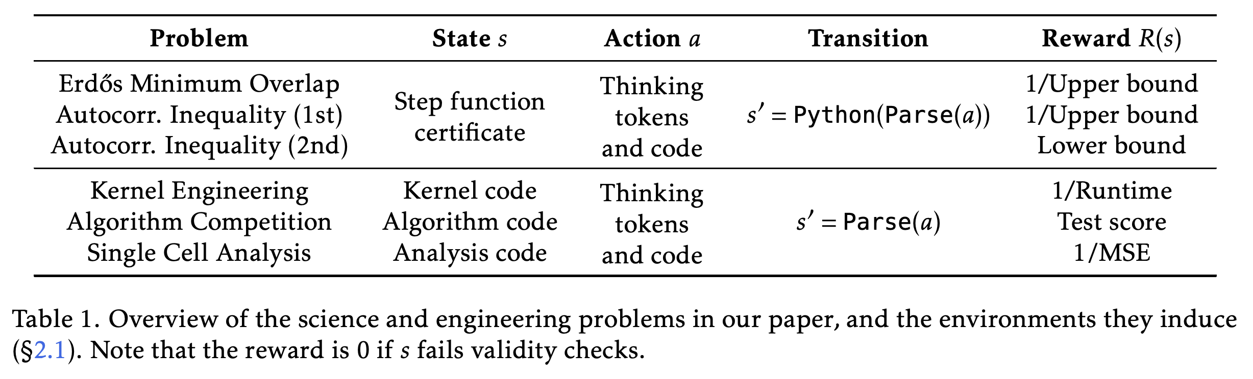
The preliminaries formulate each problem as an environment shared by search methods and learning methods. Table 1 identifies the candidate state, generated action, transition, and continuous reward for the mathematical, kernel, algorithm, and single-cell applications.

2.1 Discovery Problem

A problem description d conditions an LLM policy, a state s represents a candidate solution, and an action contains code with optional thinking tokens. A discovery occurs when R(s) > r_sota, where r_sota is the reward of the best-known solution; candidates that fail validity checks receive zero reward.

For mathematical problems, parsed Python code is executed to produce a numerical construction.
For kernel, algorithm, and analysis tasks, parsing the generated code produces the next candidate implementation.
The explicit environment has one timestep, while reuse of previous candidates effectively extends trajectories.

States, actions, transitions, and rewards for the mathematical, kernel, algorithm, and single-cell environments.

2.2 Search Methods

Best-of-N samples independent attempts from a frozen policy, usually starting from an empty or trivial solution to reduce anchoring on prior art. State reuse maintains a buffer and selects previous candidates as starting points; state-action reuse also supplies reasoning or intermediate information from earlier actions.

Starting from scratch supports exploration but can leave promising partial solutions insufficiently developed.
Evolutionary search methods such as AlphaEvolve use state-action reuse with hand-crafted mutation, crossover, fitness, and diversity heuristics.

3 Learning to Discover at Test Time

Algorithm 1 alternates candidate selection, generation, evaluation, buffer insertion, and policy updating. Its two configurable subroutines are reuse and train, and its output is the highest-reward candidate encountered during the run rather than the final policy.

3.1 Naive RL at Test Time

Naive test-time RL maximizes expected reward while restarting each attempt from the empty state. The paper identifies three mismatches with discovery: small record improvements can receive weak reward distinctions, independent restarts restrict the effective horizon, and expected-reward optimization can favor safe actions over rare record-setting outcomes.

The illustrative kernel example contrasts a 2000 µs record with a difficult 1900 µs improvement that receives only a small reward difference without additional shaping.
Reuse also requires exploration: repeatedly expanding a few high-reward states can suppress diversity.

3.2 TTT-Discover

The entropic objective is Jβ(θ) = E_s[log E_a[exp(β(s)R(s,a))]], which exponentially emphasizes high-reward actions. Its policy-gradient weights are normalized exponential rewards, with a mean baseline and a KL penalty against the initial policy; β(s) is adapted separately for each starting state.

Large β concentrates updates on the best outcomes but can destabilize early training; small β can make advantages vanish when later improvements become narrow.
Appendix A.1 chooses β by constraining the KL divergence of an auxiliary reward-tilted distribution, using γ = ln(2).
The objective favors high-reward outcomes but does not provide a finite-budget guarantee of discovering a new record.

PUCT-inspired reuse prioritizes candidates using their best observed child reward, a reward-rank prior, and an exploration bonus for less-visited lineages. Appendix A.2 specifies score(s) = Q(s) + c·scale·P(s)·√(1+T)/(1+n(s)), where scale is the archive reward range.

Q(s) uses the maximum child reward rather than the mean, reflecting the goal of finding the best continuation.
The archive retains the top-2 children per expanded parent and the top-1000 states globally, while preserving initial seeds.
Visitation counts propagate to ancestors, and ancestors and descendants of a selected state are blocked within the current batch to encourage lineage diversity.

3.3 Implementation Details

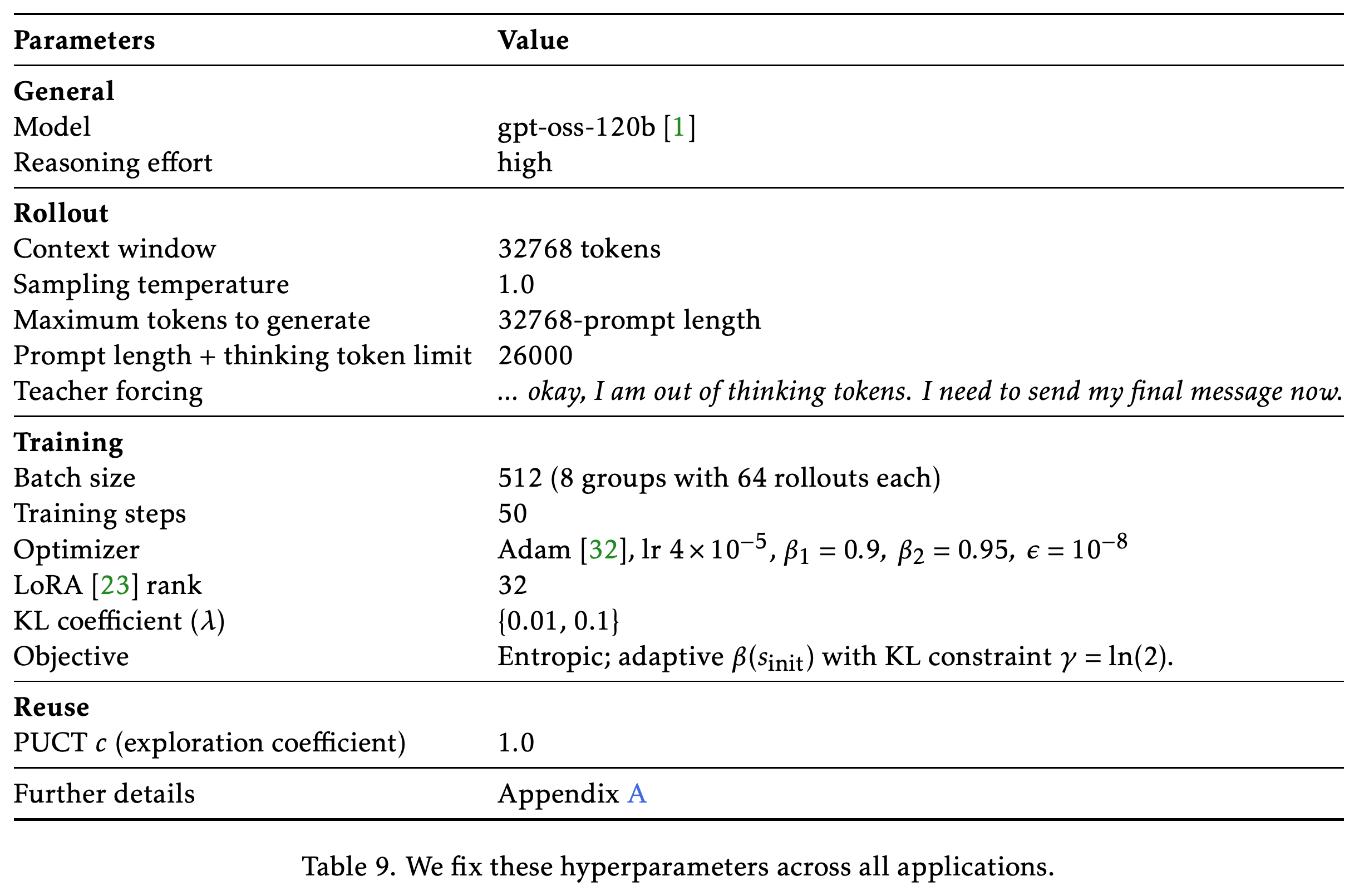
The standard implementation uses gpt-oss-120b on Tinker, rank-32 LoRA, and 50 training steps. Each step samples eight groups of 64 rollouts, sharing a starting state and context within each group, then takes one gradient step on the full 512-rollout batch with sampler/learner importance-ratio correction.

Reasoning effort is high, and the Tinker context window is 32,768 tokens. The usual prompt-plus-thinking limit is 26,000 tokens, reserving space for final code.
Table 9 lists temperature 1.0, Adam learning rate 4 × 10⁻⁵, β1 = 0.9, β2 = 0.95, ε = 10⁻⁸, and PUCT exploration coefficient 1.0.
The approximately $500 Tinker estimate assumes a 3000-token average prompt and 16,000 sampled tokens per rollout; it is not an itemized total covering candidate-execution infrastructure.

Default model, rollout, optimizer, LoRA, KL, adaptive-objective, and PUCT hyperparameters.

4.1 Mathematics

The applications compare against human experts and previous AI results, with Best-of-25600 matching TTT-Discover’s model and sampling budget. OpenEvolve also receives 25,600 samples where evaluated, but its growing prompts frequently cause truncation under the shared context-window limit.

Mathematical solutions are explicit numerical constructions that certify bounds, rather than free-form proof claims.
Mathematical actions optimize step functions or geometric configurations, and validity checks gate their rewards. The main text describes random valid initialization rather than initialization from the best-known construction.
The main text specifies a 10-minute mathematical action limit, whereas Appendix B describes verifier timeouts of up to 1100 seconds for the inequality and Erdős’ tasks.

4.1.1 Erdős’ Minimum Overlap Problem

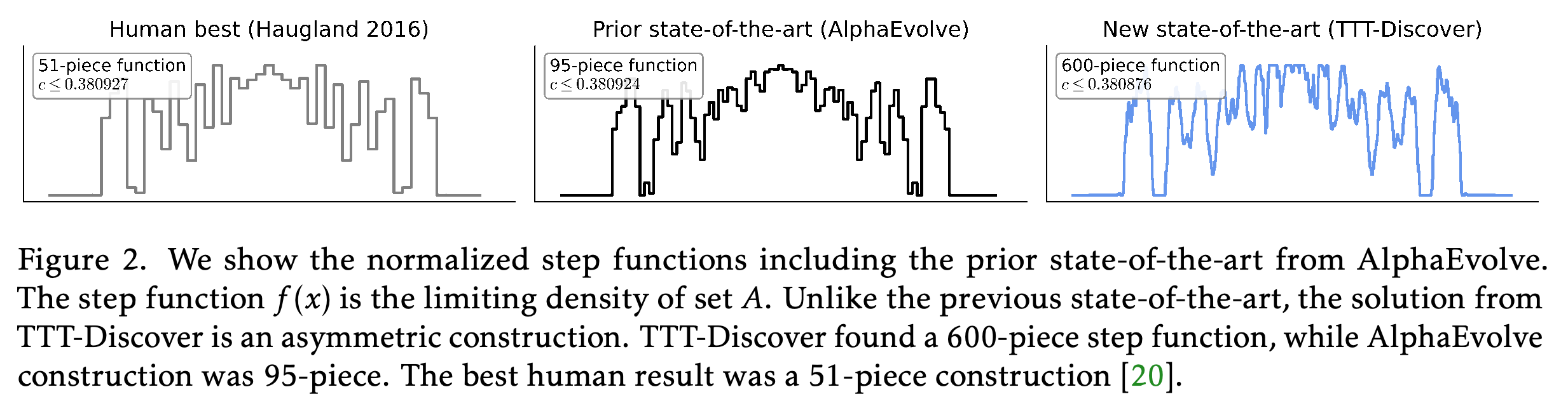
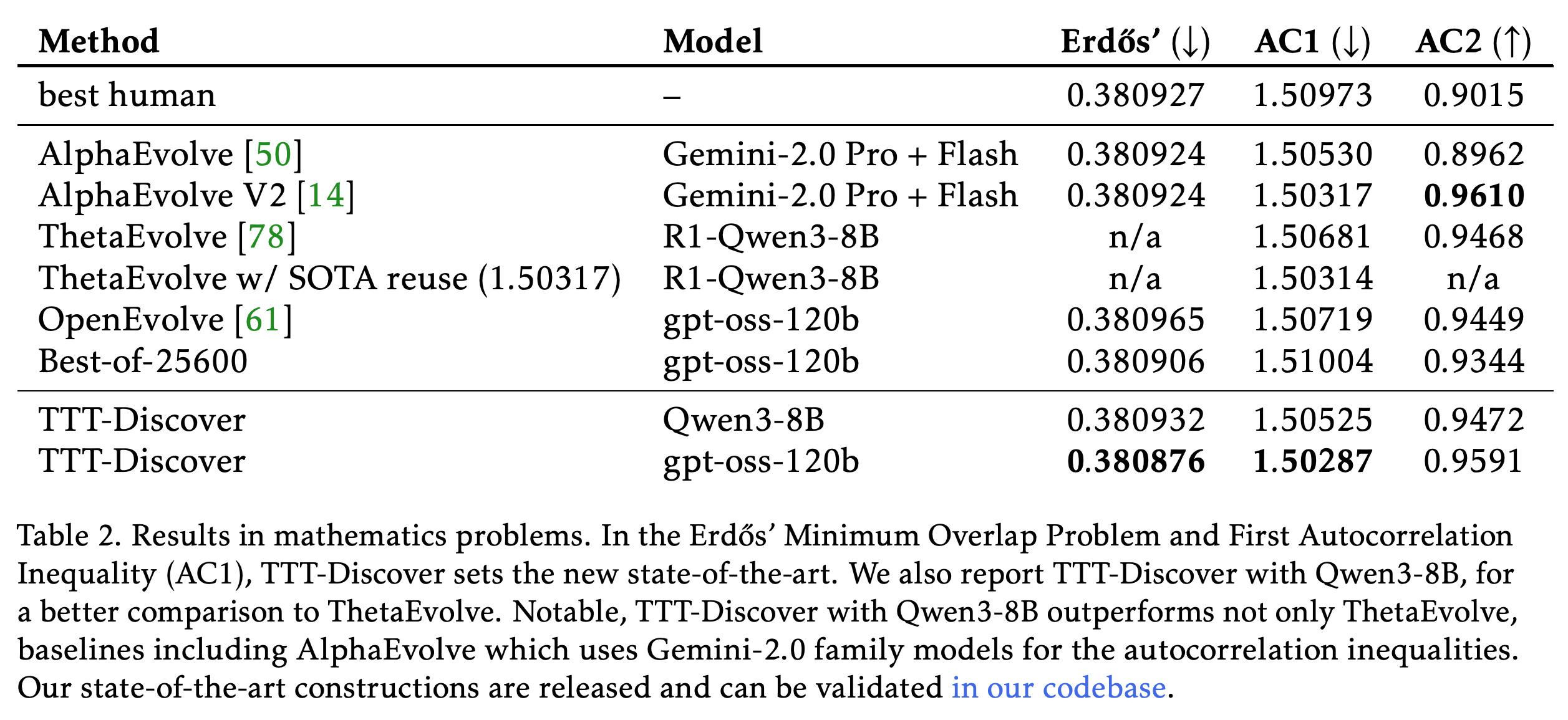
Erdős’ Minimum Overlap Problem partitions {1,2,…,2n} into equally sized sets A and B and minimizes the maximum number of cross-set differences at any offset. TTT-Discover certifies an upper bound of 0.380876 for c = lim M(n)/n, improving on AlphaEvolve’s 0.380924 and Haugland’s 0.380927.

The certificate is a 600-piece asymmetric density function with values in [0,1] and integral 1. Figure 2 compares it with 51-piece human and 95-piece AlphaEvolve constructions.
The discovered program combines FFT-accelerated gradient descent, random hill climbing, simulated annealing, and projection onto the feasibility constraints.
Table 2 also reports 0.380906 for Best-of-25600, which independently improves the previous AI record; TTT-Discover improves further.

Normalized density-function certificates for Erdős’ Minimum Overlap Problem from Haugland, AlphaEvolve, and TTT-Discover.

4.1.2 Autocorrelation Inequalities

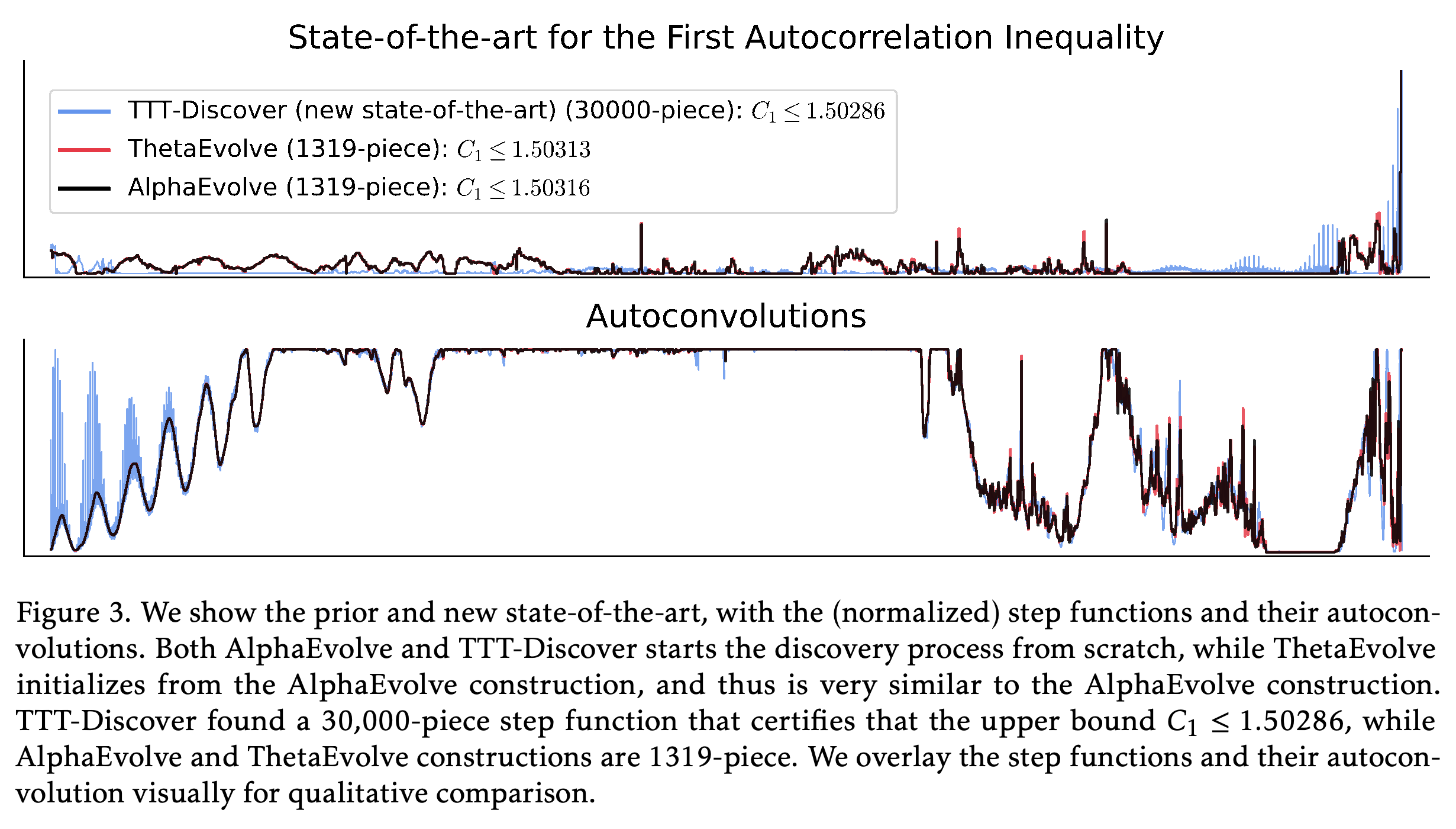
The first autocorrelation inequality seeks a tight upper-bound certificate for C1 using nonnegative functions supported on [−1/4,1/4]. Any valid f certifies C1 ≤ ||f∗f||∞/||f||₁². TTT-Discover finds a new 30,000-piece construction from scratch; the results text and Figure 3 report C1 ≤ 1.50286, whereas Table 2 reports 1.50287.

The search progresses from gradient-based optimization to linear programming, then focuses optimization on convolution constraints close to their maximum.
Later heuristics include selecting the top K convolution positions for the LP and computing gradients from multiple near-maximum positions.
Figure 3 reports ThetaEvolve and AlphaEvolve bounds of 1.50313 and 1.50316, while Table 2 reports 1.50314 and 1.50317 for ThetaEvolve with SOTA reuse and AlphaEvolve V2. Both presentations show an improved TTT-Discover bound.

Step functions and autoconvolutions for the first autocorrelation inequality, including the 30,000-piece TTT-Discover certificate.

The second inequality defines C2 = sup_f≥0 ||f∗f||₂²/(||f∗f||₁||f∗f||∞); a construction with ratio r certifies C2 ≥ r. Table 2 reports 0.9591 for TTT-Discover, below AlphaEvolve V2’s 0.9610, so this task produces no new record.

With Qwen3-8B, TTT-Discover obtains AC1 = 1.50525 and AC2 = 0.9472, improving on ThetaEvolve’s values of 1.50681 and 0.9468 without SOTA initialization.
This is not an identical-model comparison: ThetaEvolve uses DeepSeek-R1-0528-Qwen3-8B, unavailable on Tinker, whereas TTT-Discover uses Qwen/Qwen3-8B.
ThetaEvolve uses 65 steps of 512 rollouts, versus 50 for TTT-Discover. ThetaEvolve’s AC1 result with SOTA reuse, 1.50314, is stronger than the Qwen3-8B TTT-Discover result.

Mathematical bound comparisons across human constructions, previous AI systems, matched-budget baselines, and TTT-Discover.

4.1.3 Circle Packing

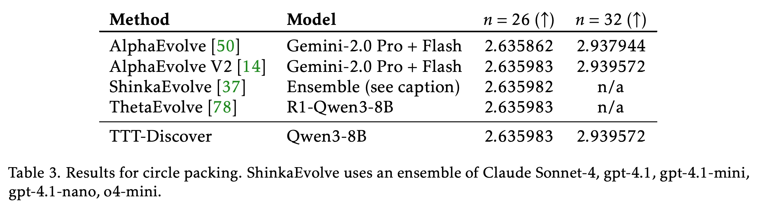
Circle packing maximizes the sum of radii of n non-overlapping circles inside a unit square. Table 3 reports that Qwen3-8B TTT-Discover matches the best-known sums, 2.635983 for n = 26 and 2.939572 for n = 32, without improving either record.

The generated programs initialize grid-based arrangements, then optimize centers and radii using sequential least squares programming.
Boundary and pairwise non-overlap constraints determine validity. The paper contrasts these geometric initializations with ShinkaEvolve’s simulated-annealing-based initialization.

Circle-packing sums of radii for n = 26 and n = 32 across previous systems and TTT-Discover.

4.1.4 Expert Review

Human Expert Review — Prof. Davide Torlo (Università di Roma La Sapienza) explains why the Erdős’ and AC1 certificates are directly checkable. Verification evaluates the relevant quantities at discrete points determined by the piecewise-constant functions’ step sizes and checks the norm constraints. This supports the bound improvements without establishing closed-form optima.

4.2 Kernel Engineering

Kernel Engineering evaluates retrospective GPUMode TriMul and DeepSeek MLA-Decode competitions using correctness checks and rewards proportional to inverse geometric-mean runtime. TriMul training evaluates kernels on H100, while MLA-Decode training uses H200 because MI300X is unavailable at scale on Modal.

Table 4 reports TriMul runtimes of 2198.2 µs on A100, 1161.2 µs on H100, 914.2 µs on B200, and 1555.7 µs on AMD MI300X.
The corresponding best-human runtimes are 4531.5, 1371.1, 1038.9, and 2515.8 µs, respectively. Training uses one H100-based reward, but Appendix C describes target-hardware selection for the final kernels.
A100 and H100 values come from official submissions. B200 and MI300X results use organizer-verified replicated infrastructure with 10 trials and 95% confidence intervals because server problems prevented official submissions.

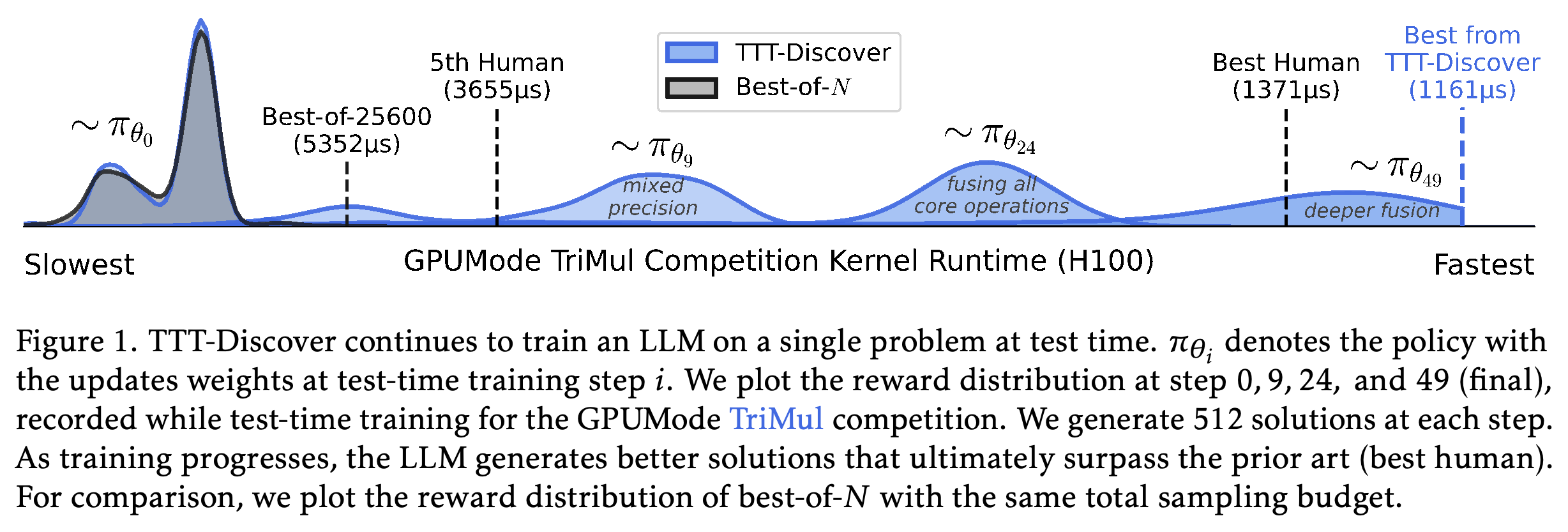
The TriMul implementation reduces memory traffic and launch overhead through operation fusion, stores intermediate activations in FP16, and delegates the large matrix multiplication to cuBLAS/rocBLAS. Figure 1 associates the changing rollout distribution with mixed precision, fusion of core operations, and deeper fusion as training proceeds.

Appendix C identifies fusion of output LayerNorm and gating with output projection as a possible source of the advantage over the best human H100 kernel.
The generated H100 kernel performs less block-size autotuning than the human implementation, which the authors identify as a limitation.

TriMul H100 rollout distributions at training steps 0, 9, 24, and 49, compared with matched-budget Best-of-N and human runtime references.

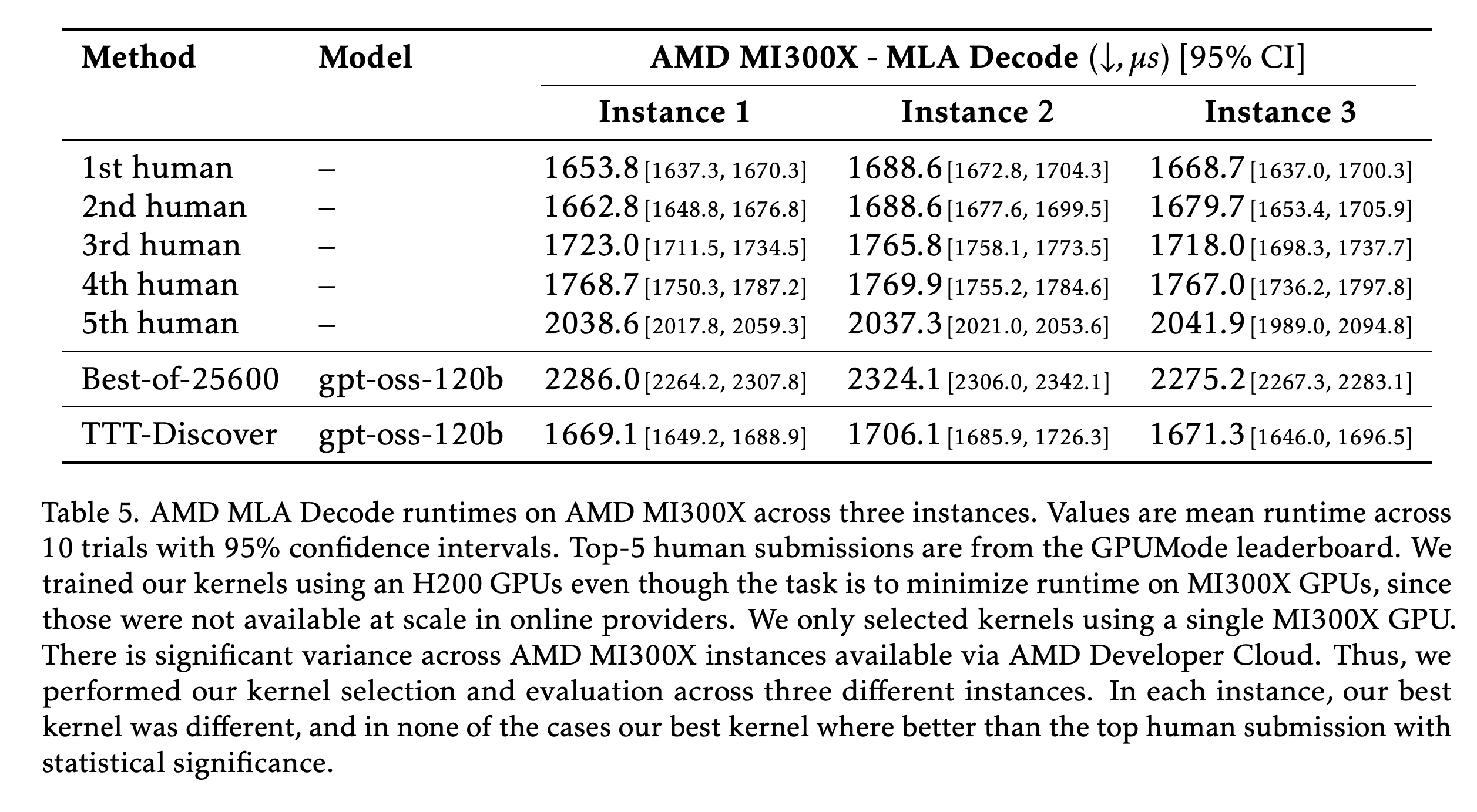
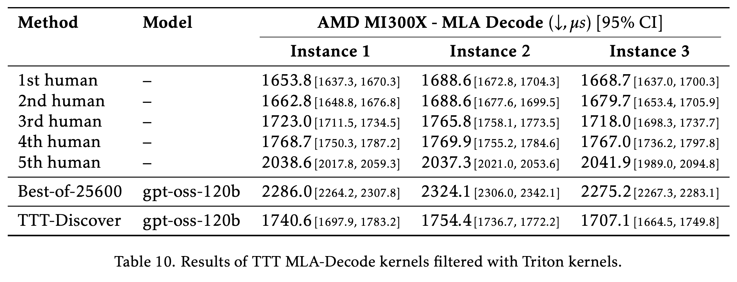
MLA-Decode produces no new record: Table 5 reports 1669.1, 1706.1, and 1671.3 µs across three MI300X instances, with no statistically significant advantage over the top human submission. The fastest generated implementations mainly use a particular torch.compile() configuration rather than explicit Triton kernels for fine-grained optimization.

Cross-instance runtime variation complicates selection. Table 5 states that the best generated kernel differs across the three instances.
Table 10 separately filters for explicit Triton implementations, reporting 1740.6, 1754.4, and 1707.1 µs, again without a human-beating record.

MLA-Decode runtimes in µs across three AMD MI300X instances, measured over 10 trials with 95% confidence intervals.

MLA-Decode runtimes for generated kernels explicitly using Triton across three AMD MI300X instances.

4.2.1 Expert Review

Human Expert Review — Matej Sirovatka, Alex Zhang, Mark Saroufim (GPUMode) supports the TriMul strategy of fusing memory-bound pointwise operations and using library matrix multiplication. The organizers also caution that FP16 activation storage, although valid under competition tolerances, could introduce numerical stability problems in full workloads.

4.3 Algorithm Engineering

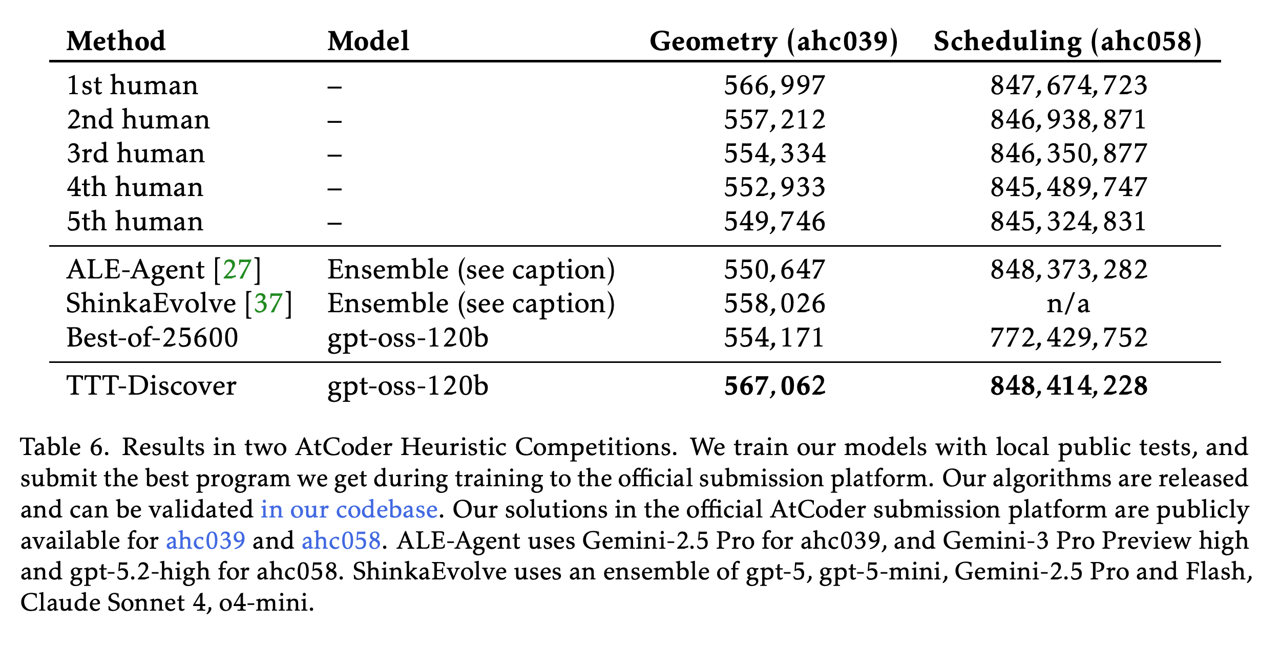
Algorithm Engineering evaluates ahc039 (Purse Seine Fishing) and ahc058 (Apple Incremental Game) through ALE-Bench, training on locally generated public cases and evaluating selected programs on official hidden tests. Valid C++ programs must satisfy the 2-second time limit and 1024MB memory limit.

AHC039 starts from the ALE-Agent-derived program also used by ShinkaEvolve; AHC058 starts from scratch.
Table 6 reports 567,062 for AHC039 versus the best human’s 566,997 and ShinkaEvolve’s 558,026.
AHC058 reaches 848,414,228 versus ALE-Agent’s 848,373,282 and the best human’s 847,674,723. These are retrospective first-place-equivalent scores, not live contest victories.

Official retrospective scores for Geometry (ahc039) and Scheduling (ahc058), compared with human and AI submissions.

The AHC039 solution scores candidate rectangles with prefix sums, constructs a connected union, and refines it through simulated annealing under perimeter and vertex constraints. The AHC058 solution combines greedy initialization, short beam search, simulated annealing, cached intermediate states, and local cleanup to optimize production-upgrade schedules.

AHC039 annealing uses add, remove, replace, expand, shrink, and slide moves.
AHC058 estimates the future production value of upgrades to guide greedy choices and pruning, while recomputing only modified portions of a plan.

4.4 Single Cell Analysis

Single Cell Analysis optimizes the OpenProblems denoising task, which evaluates predictions against held-out molecules obtained through binomial sampling. TTT-Discover starts from MAGIC code and trains on Pancreas, with final results evaluated on held-out PBMC and Tabula Muris Senis Lung datasets.

Training reward is the normalized MSE score, subject to a normalized Poisson-score constraint and a 400-second execution limit. The reported benchmark Score instead averages normalized MSE and Poisson scores.
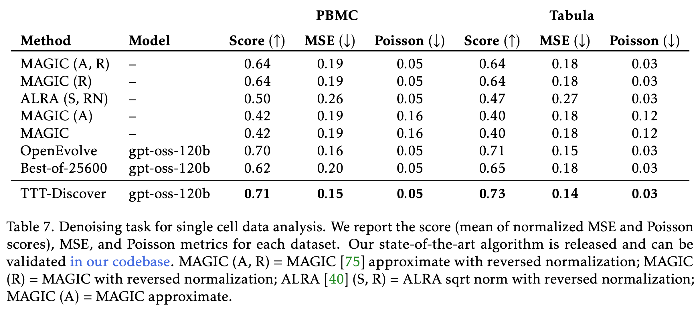
Table 7 reports PBMC Score 0.71 and MSE 0.15, versus MAGIC with reversed normalization at 0.64 and 0.19.
On Tabula, TTT-Discover reaches Score 0.73 and MSE 0.14, versus MAGIC with reversed normalization at 0.64 and 0.18. Poisson losses remain 0.05 and 0.03 on the respective datasets at the displayed precision.

Single-cell denoising scores, MSE, and Poisson losses on held-out PBMC and Tabula datasets.

The generated denoiser adds gene-adaptive transform ensembling, low-rank SVD refinement, and log-space polishing that directly targets the benchmark metric. The section’s Disclaimer limits the claim to benchmark performance: better metrics do not guarantee biological validity for downstream tasks.

4.4.1 Expert Review

Human Expert Review — Prof. Eric Sun (MIT) describes the changes as consistent with MAGIC’s smoothing-based approach and empirically beneficial on the reported metrics. He calls for evaluation on biologically relevant tasks because improved denoising scores may not translate into better biological insights.

4.5 Ablations

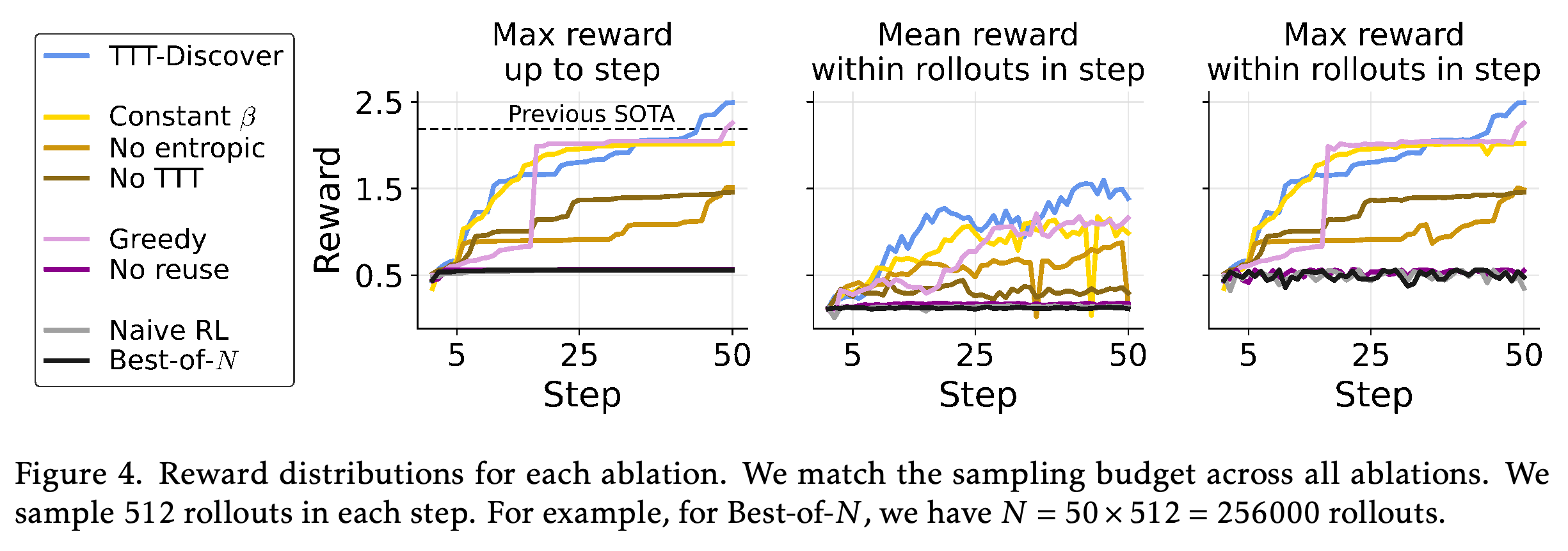
TriMul ablations separate the training objective from the reuse mechanism under matched sampling budgets. Table 8 reports 1203.10 µs for the full method, 1483.83 µs with constant β = 2, 1985.67 µs with expected-reward training, and 2060.70 µs with PUCT reuse but no training.

Replacing PUCT with ε-greedy reuse at ε = 0.1 gives 1328.89 µs, while removing reuse gives 5274.03 µs.
Naive test-time RL reaches 5328.73 µs, close to Best-of-N’s 5352.36 µs.
These runtimes use the authors’ evaluator, not the official leaderboard, and should not be conflated with Table 4’s 1161.2 µs.

TriMul H100 best-kernel runtimes for training-objective and reuse ablations under the authors’ evaluator.

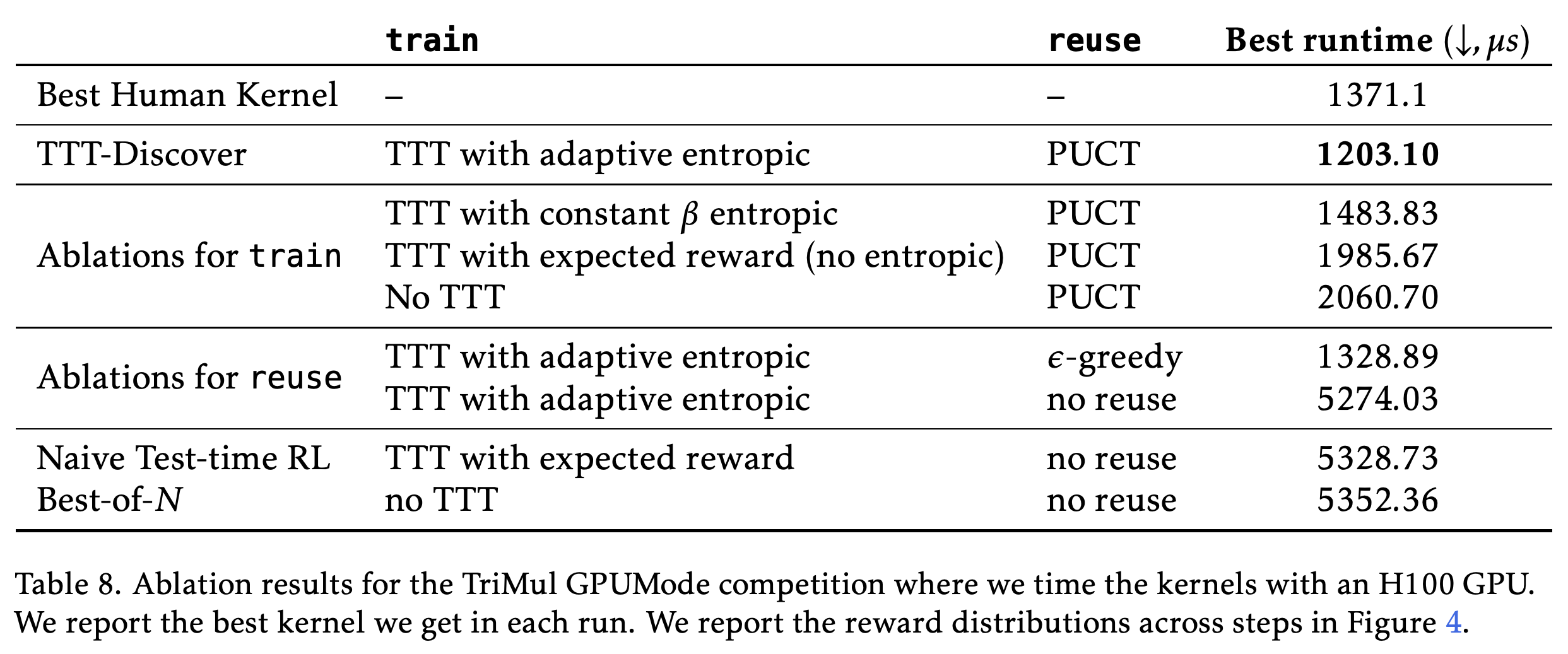
Figure 4 shows continued improvement with adaptive entropic training, diminishing late improvements with constant β, and little progress without reuse. The ablations support contributions from both learning and candidate reuse, but report the best kernel from each run without repeated-run uncertainty estimates.

The authors acknowledge that task-specific schedules, hyperparameter interactions, and additional tuning could improve the ablated configurations.
Figure 4’s caption prints N = 50 × 512 = 256000. The stated step and batch counts imply 25,600, consistent with the main experimental protocol.

Cumulative maximum, per-step mean, and per-step maximum rewards for the TriMul ablations over training.

Related Works situates TTT-Discover within continual learning and instance-specific test-time training. It distinguishes adaptation to the current discovery problem from training on one example to improve generalization and from adapting collectively across an entire test set.

5.1 Continual Learning

Conventional continual learning studies evolving data distributions while preserving performance on earlier tasks or data. TTT-Discover also updates a model after its initial training, but retention across a changing task sequence is not its primary objective.

5.2 Test-Time Training

Test-Time Training formulates a potentially different learning problem from each individual test instance. TTT on Nearest Neighbors: Larger Effective Capacity explains how local training on retrieved examples increases effective capacity, allowing the model to specialize to the current input.

Historical examples include locally weighted regression, local learning, KNN-SVM, and dynamic evaluation.
Recent variants use neighbor-based fine-tuning or RL for language reasoning and visual-motor tasks.

TTT for Novel Instances: Better Generalization extends adaptation to relevant data generated from the test instance, including self-supervised auxiliary tasks and targeted curricula. Concurrent systems MiGrATe, ThetaEvolve, and EvoTune combine per-instance updates with replay or reuse; TTT-Discover emphasizes the best discovered artifact through entropic training and maximum-based PUCT.

AlphaProof generates easier related problems for RL, while ARC-AGI test-time training augments few-shot demonstrations for supervised adaptation.
The section also discusses test-time policy gradients applied to token representations with model-based evaluation, and earlier per-instance neural policy optimization for combinatorial problems such as TSP.
The paper’s repeated claim of a same-model, same-budget ThetaEvolve comparison is qualified by Section 4.1.2: the reported runs use different Qwen variants and 50 versus 65 steps.

5.3 RL on One Example

One Example RL trains on a single example from a training dataset and evaluates generalization to other examples. TTT-Discover instead trains on the test problem itself, where solving that same problem is the objective.

5.4 RL on the Test Set

TTRL adapts on an entire test set using majority-vote pseudo-labels for reward estimation. TTT-Discover uses one problem with a continuous, verifiable reward and searches for an exceptional candidate rather than improved average accuracy across multiple problems.

6 Future Work

Future Work identifies extending the method to sparse or binary rewards and non-verifiable domains as the main research direction. The current experiments do not establish effectiveness in those settings.

Appendix

A Training details specifies KL coefficient 0.1 for almost all applications and 0.01 for algorithm engineering. A.1 Entropic utility objective chooses β by bisection to satisfy (\operatorname{KL}(q_\beta|u)=\gamma) with γ = ln(2), then computes leave-one-out entropic advantages; the appendix states invariance to positive reward scaling and additive shifts. A.2 PUCT Prioritization specifies the reward-range-scaled exploration bonus, rank prior, maximum-child statistic, ancestor visitation updates, top-2/top-1000 archive retention, and within-batch lineage blocking.
B Mathematics includes B.1 Circle Packing programs: Circle Packing (n = 26) initializes five rows and jointly optimizes centers and radii with SLSQP, while Circle Packing (n = 32) initializes 30 hexagonally arranged circles plus two extra circles, optimizes boundary and distance constraints, and falls back to its initial arrangement after optimization or validation failure. B.2 Autocorrelation Inequalities describes repeated random-height initial sequences, input validation, the discrete AC1 upper-bound calculation, and piecewise-linear integration for AC2. B.3 Erdős’ initializes 40–100 perturbed values around 0.5 and rejects sequences longer than 1000; the inequality and Erdős’ evaluators use 1 GB, 2 CPUs, and timeouts of up to 1100 seconds.
C Kernel engineering describes the initial TriMul matrix-multiplication example and the preliminary model-generated, unoptimized MLA-Decode kernel; C.1 Kernel evaluation details documents competition-matched correctness and timing checks, official A100/H100 submissions, and organizer-reviewed replicated environments for the other hardware. H100 selection uses the top 20 training candidates; other targets use the top 20 training candidates plus 20 random correct kernels every 10 steps, evaluate selected candidates three times on target hardware, and choose the smallest average runtime. C.2 Analysis of best generated kernels and TriMul H100 provide the fused FP16 implementation and discuss memory-access improvements and limited autotuning; C.3 TTT MLA-Decode kernels filtered with Triton kernels reports the slower explicit-Triton results.
D Algorithm Engineering trains on 150 generated cases with seeds 0 through 149 using yimjk/ale-bench:cpp20-202301, requiring correctness and execution within 2 seconds on every case, then submits the top three locally scored programs as C++23 (GCC 15.2.0). AHC039 uses ShinkaEvolve’s relative-placement performance metric, while AHC058 uses the contest score directly. AHC039 reduces the prompt-plus-thinking limit to 22000 tokens; AHC058 uses 25000 and learning rate 2 × 10⁻⁵, and both use KL coefficient 1 × 10⁻².
E Single cell analysis requires normalized Poisson performance between 0.97 and 1, increases memory to 3GB, and limits execution to 400 seconds; training optimizes normalized MSE, whereas the benchmark score averages normalized MSE and Poisson performance. TTT-Discover and Best-of-25600 use a 20,000-token generation limit, and OpenEvolve runs for 25,600 samples but selects its best program from before sample 17,000 because later archive entries increasingly time out. Denoising provides magic_denoise and helper functions for variance-stabilizing transforms, gene-dependent diffusion and blending, transform ensembling, low-rank SVD refinement, and log-space polishing; final evaluation uses default parameters.
F Prompts contains sample-step templates rather than complete standalone evaluators. Prompt used for the first autocorrelation inequality supplies a prior LP-based approach, previous bounds and logs, a 1000-second search budget, and the propose_candidate entrypoint; Prompt used for the second autocorrelation inequality describes explore–refine–upscale search and requires construct_function; Prompt used for the Erdős’ specifies h on [0,2], values in [0,1], integral 1, correlation-based evaluation, and a run entrypoint. Prompt used for TriMul supplies the PyTorch forward reference, input cases, mixed-precision requirements, and custom_kernel for Triton 3.3.1 on H100; Prompt used for MLA-Decode supplies the attention and KV-cache reference, custom_kernel, and Triton 3.4.0/H200 requirements with torch.compile() allowed; Prompt used for the AHC039 specifies polygon constraints and fishing scores, Prompt used for the AHC058 specifies hierarchical production upgrades and output actions, and Prompt used for Denoising specifies magic_denoise, held-out-molecule metrics, normalization guidance, and the Poisson constraint; several verifier, previous-code, and resource fields remain placeholders.

Brief Thoughts

The contribution is the joint design of test-time policy updates and candidate reuse for a best-artifact objective, supported by checkable mathematical constructions, external evaluations where available, and component ablations. The evidence remains limited to continuous, verifiable rewards: baseline context and timeout constraints complicate comparisons, the ThetaEvolve comparison changes model variants and budgets, and biological validity is untested. The reported failures on AC2, circle packing, and MLA-Decode are essential to interpreting the method’s scope.