Summary explanation: Marigold V2: Revisiting Diffusion Transformers for Monocular Depth Estimation

Contents

• Summary
• 1 Introduction
• 3 Method
  • 3.2 Diffusion Transformer Adaptation
  • 3.3 Semantic Feature Regularization with iREPA
  • 3.4 Stage-2 Refinement with SinkLoss
• 4 Experiments
  • 4.3 Zero-Shot Affine Depth Estimation
  • 4.5 Analysis and Ablation Studies
• 5 Other Dense Regression Tasks
  • 5.1 Depth Completion
• Appendix
• Brief Thoughts

This article explains the key points of Marigold V2: Revisiting Diffusion Transformers for Monocular Depth Estimation.

• 2026-09-08 (arXiv), ACM Transactions on Graphics
• Pavlovic, Igor, Wandel, Thiemo, Obukhov, Anton, Bartolomei, Luca, Davydov, Andrey, Tosi, Fabio, Poggi, Matteo, Süsstrunk, Sabine, Dai, Dengxin.
• EPFL, Switzerland, HUAWEI Bayer Lab, Switzerland, University of Bologna, Italy
• Paper
• Github
• Project Page

Read this article in Korean

Summary

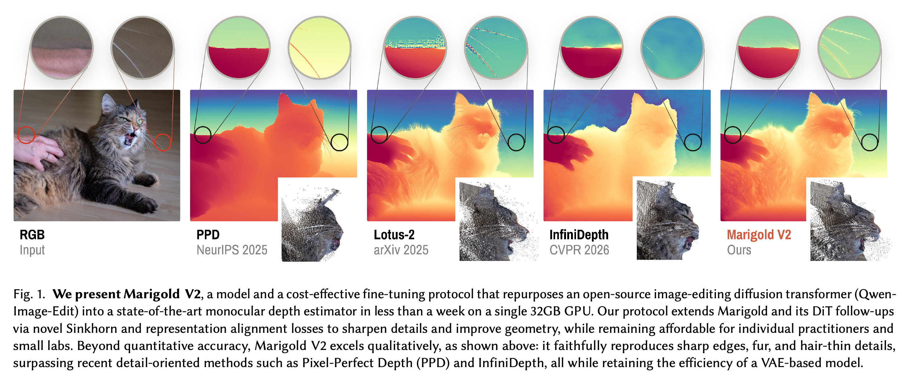
• Marigold V2 repurposes Qwen-Image-Edit-2509, an image-editing diffusion transformer, as a single-step affine-invariant monocular depth estimator. The two-stage protocol combines 4-bit QLoRA adaptation, iREPA-depth semantic regularization, and SinkLoss refinement; the final Stage-1 run uses 74K training images and a single 32GB GPU for slightly more than five days.

Shows a cat image with enlarged regions of depth predictions from PPD, Lotus-2, InfiniDepth, and Marigold V2. The displayed Marigold V2 output retains fur texture and narrow boundaries more clearly than the shown alternatives.

1 Introduction

Single-image depth estimation is intrinsically ambiguous, and discriminative models remain limited by the coverage and quality of annotated depth data, particularly for non-Lambertian, transparent, and reflective surfaces. Diffusion-derived estimators exploit broad generative priors but often blur boundaries and lose high-frequency structure; the paper targets these artifacts while retaining single-pass inference.

3 Method

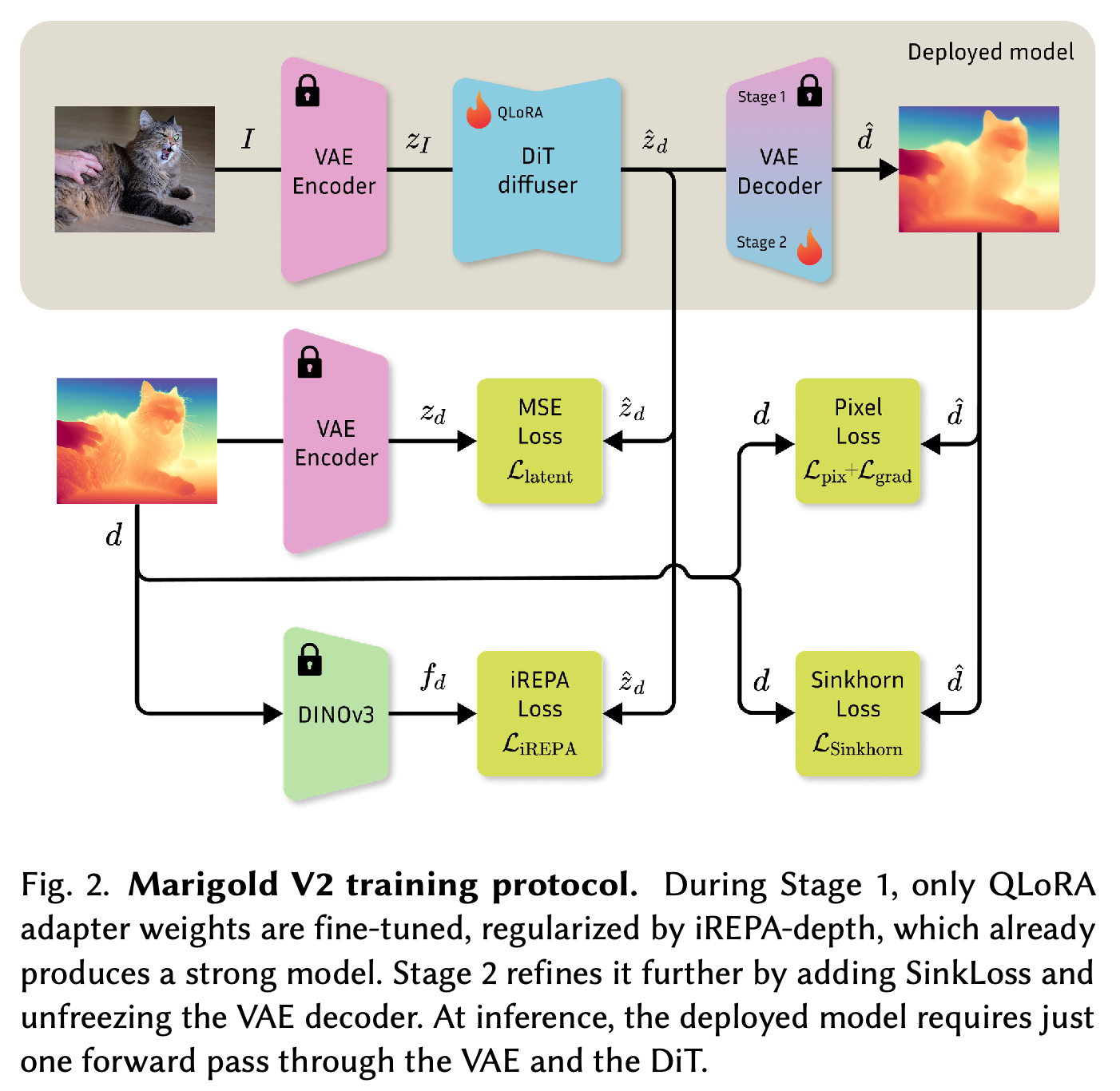
The method converts metric depth to a clipped affine-invariant normalized log-depth target using the 2nd and 98th percentiles over valid pixels, then replicates it into three grayscale channels for the image-editing backbone. Stage 1 learns RGB-latent-to-depth-latent rectified-flow regression with latent, pixel, gradient, and semantic losses, while Stage 2 handles locally ambiguous supervision around thin and transparent structures.

Depicts the two-stage protocol: Stage 1 trains QLoRA adapters with latent, pixel, gradient, and iREPA-depth losses, while Stage 2 adds SinkLoss and unfreezes the VAE decoder. Inference uses one pass through the VAE and DiT.

3.2 Diffusion Transformer Adaptation

Starting from Qwen-Image-Edit-2509, the authors quantize pretrained DiT weights to 4-bit precision and fine-tune rank-128 QLoRA adapters. At fixed timestep t = 0.5, the DiT predicts the velocity between RGB and normalized-depth VAE latents, enabling depth-latent recovery and VAE decoding in one forward pass.

3.3 Semantic Feature Regularization with iREPA

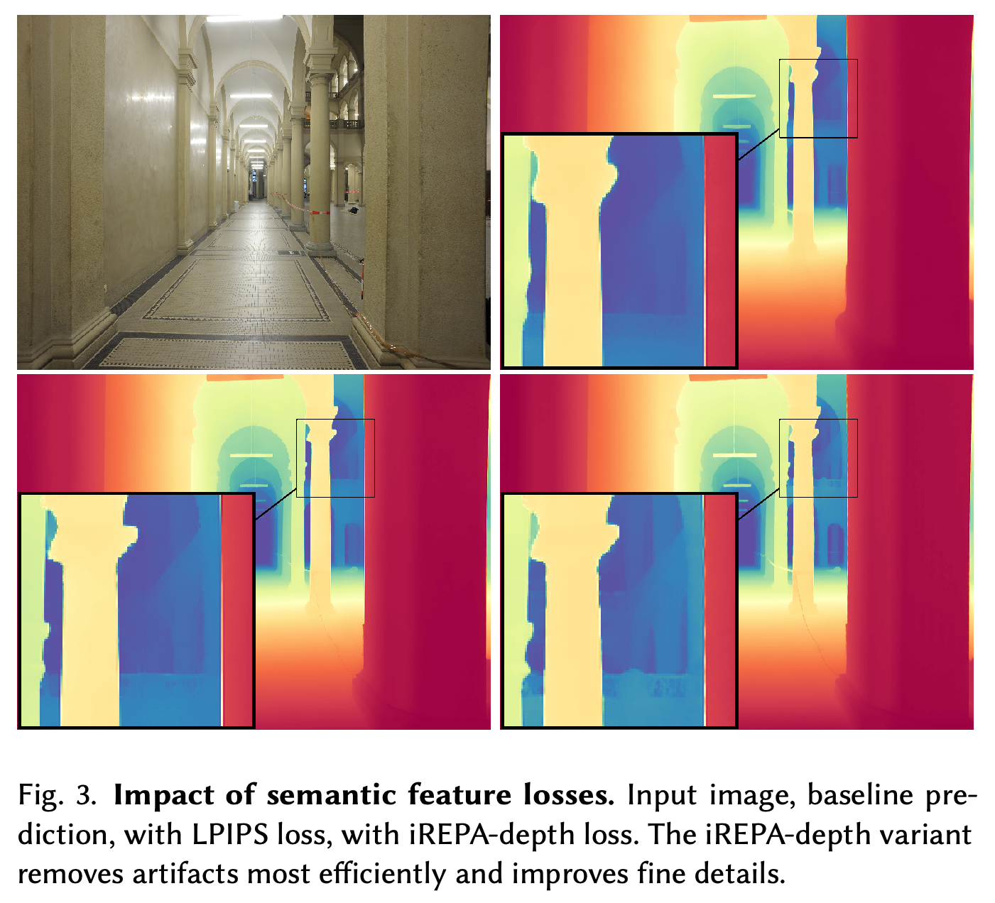
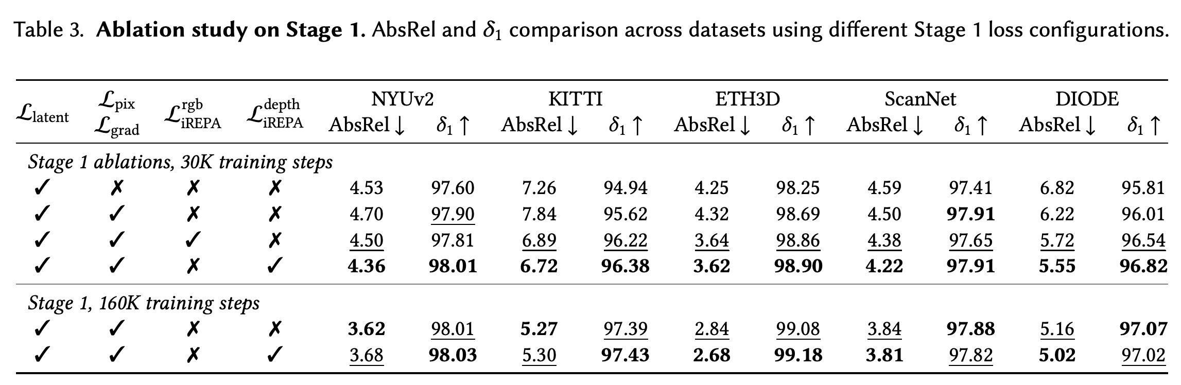
iREPA-depth regularizes internal DiT features with frozen DINOv3 features extracted from the ground-truth depth map rather than from the input RGB image. In the 30K-step ablation, depth-derived iREPA gives the strongest overall configuration; after 160K steps, its numerical advantage is smaller, although the paper reports continuing qualitative benefits in detailed regions.

Compares the input image with baseline, LPIPS-regularized, and iREPA-depth predictions. The iREPA-depth result visually removes local artifacts and better preserves structure in the corridor scene.

3.4 Stage-2 Refinement with SinkLoss

SinkLoss partitions an image into non-overlapping K×K blocks and uses entropy-regularized Sinkhorn matching between predicted and target depth values inside each block, relaxing exact pixel correspondence where labels are locally ambiguous or noisy. The implementation uses K = 5, τ = 0.1, B = 10^6, and five Sinkhorn iterations; Stage 2 also unfreezes the VAE decoder.

4 Experiments

Training samples HyperSim and vKITTI with probabilities of 90% and 10%, at 768 × 512 and 1216 × 352, respectively. All experiments use one 32GB GPU: final Stage 1 runs for 160K steps, Stage 2 adds 30K steps, and evaluation RANSAC-aligns predictions to metric ground truth before computing affine-depth metrics.

4.3 Zero-Shot Affine Depth Estimation

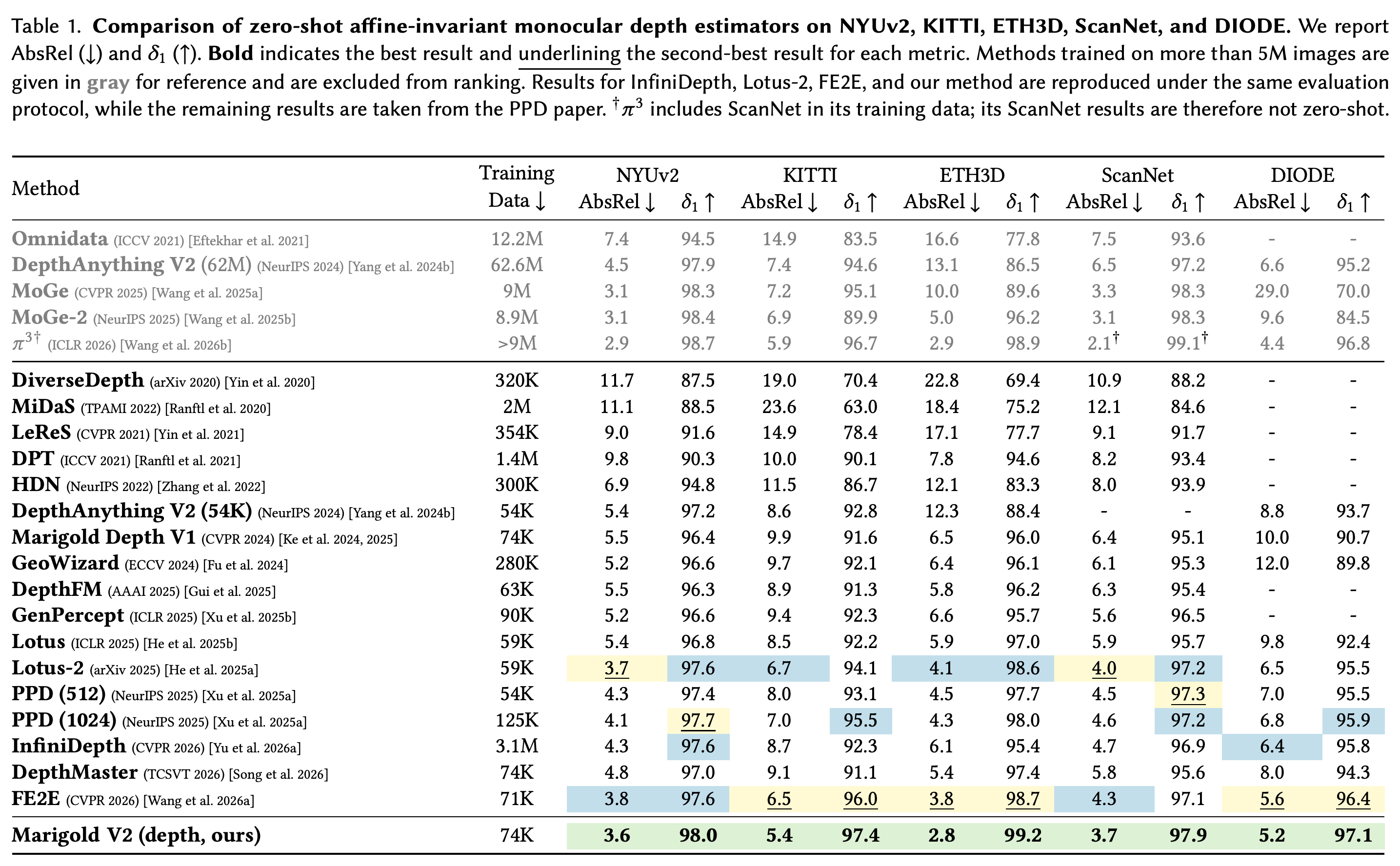
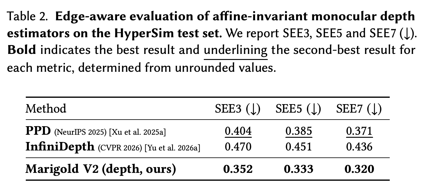
On NYUv2, KITTI, ETH3D, ScanNet, and DIODE, the Stage-2 model reports AbsRel/δ1 of 3.6/98.0, 5.4/97.4, 2.8/99.2, 3.7/97.9, and 5.2/97.1, respectively. Table 1 ranks it best across these metrics among methods trained on comparable-scale data; on HyperSim, it reports SEE3/SEE5/SEE7 of 0.352/0.333/0.320 for edge-aware evaluation.

Reports zero-shot affine-depth AbsRel and δ1 on five benchmarks. Marigold V2 records 3.6/98.0 on NYUv2, 5.4/97.4 on KITTI, 2.8/99.2 on ETH3D, 3.7/97.9 on ScanNet, and 5.2/97.1 on DIODE; these are best among the table's comparable-data methods.

Evaluates boundary quality on HyperSim with Soft Edge Error. Marigold V2 has the lowest reported SEE3, SEE5, and SEE7 values—0.352, 0.333, and 0.320—among the three listed methods.

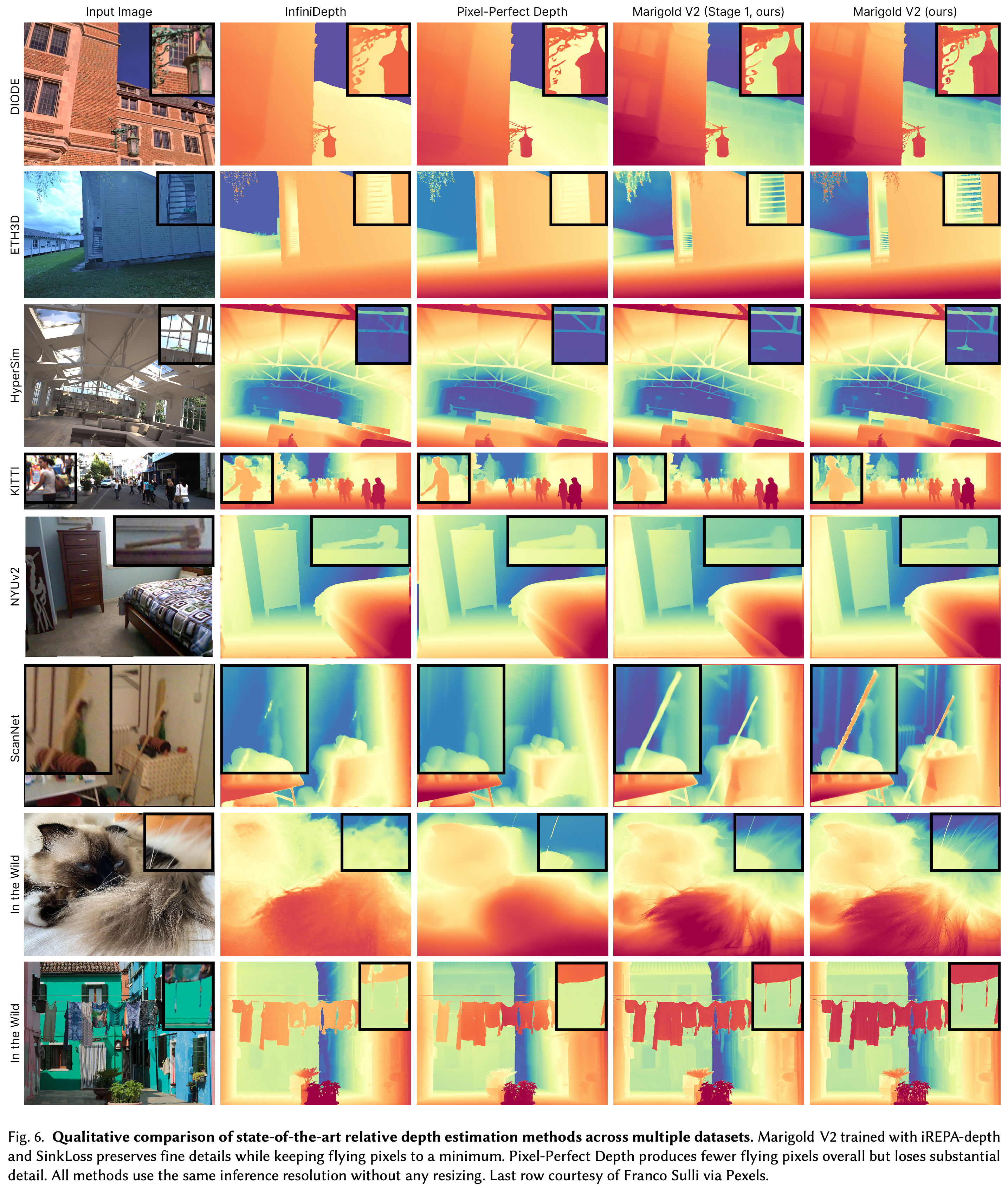
Presents relative-depth predictions on DIODE, ETH3D, HyperSim, KITTI, NYUv2, ScanNet, and in-the-wild images. The final Marigold V2 column is shown with sharper thin structures and fewer flying pixels than its Stage-1 output and the displayed baselines.

4.5 Analysis and Ablation Studies

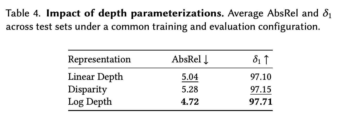
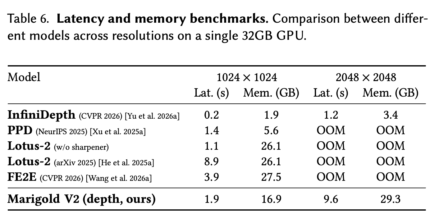
Among tested representations, normalized log-depth has the best average result, with 4.72 AbsRel and 97.71 δ1, compared with 5.04/97.10 for linear depth and 5.28/97.15 for disparity. SinkLoss improves edge-sensitive SEE metrics on Stable Diffusion V1.5, FLUX.2 klein, and Qwen-Image-Edit-2509; at 2048 × 2048, Marigold V2 runs in 9.6 s using 29.3 GB on a single 32GB GPU.

Shows Stage-1 loss ablations at 30K and 160K steps. At 30K, depth-derived iREPA is strongest overall; at 160K, the gap between iREPA-depth and the configuration without iREPA becomes smaller.

Compares linear-depth, disparity, and log-depth parameterizations under a common setting. Normalized log-depth has the best average values, 4.72 AbsRel and 97.71 δ1.

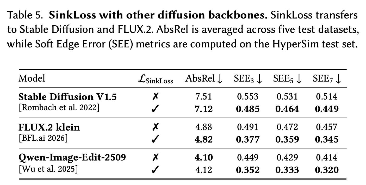
Tests SinkLoss on Stable Diffusion V1.5, FLUX.2 klein, and Qwen-Image-Edit-2509. Enabling it lowers every reported Soft Edge Error metric for all three backbones, while the average AbsRel change is small.

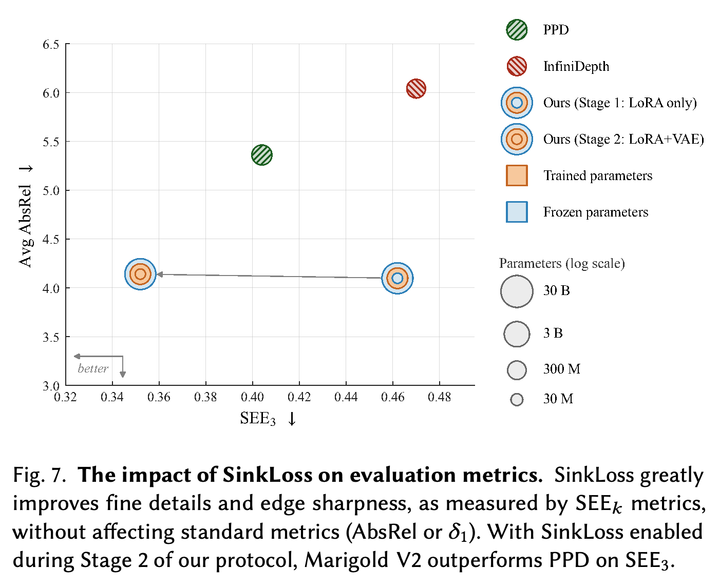
Plots average AbsRel against SEE3 and parameter scale. The Stage-2 SinkLoss point substantially improves edge error relative to Stage 1 while preserving a similar average AbsRel.

Benchmarks inference on a single 32GB GPU. Marigold V2 takes 1.9 s and 16.9 GB at 1024 × 1024, and 9.6 s and 29.3 GB at 2048 × 2048, where PPD, Lotus-2, and FE2E are reported out of memory.

5 Other Dense Regression Tasks

The authors extend the recipe to metric depth completion, see-through depth, surface-normal estimation, and albedo estimation. These experiments show that the same adaptation framework can be applied to other dense regression outputs, while the paper notes that the large image-editing backbone is not suitable for real-time use and that reflections, motion, and defocus blur remain ambiguous.

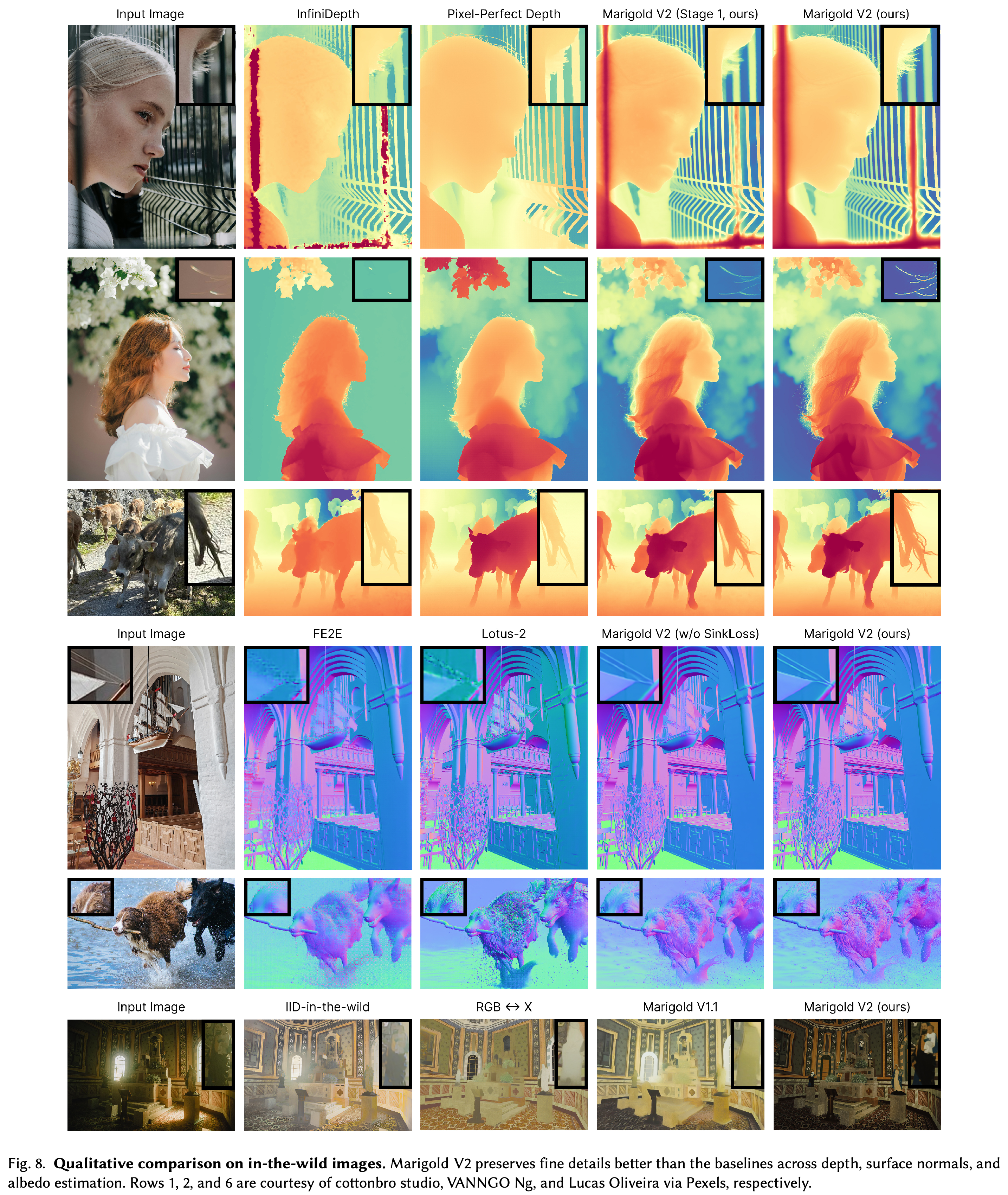
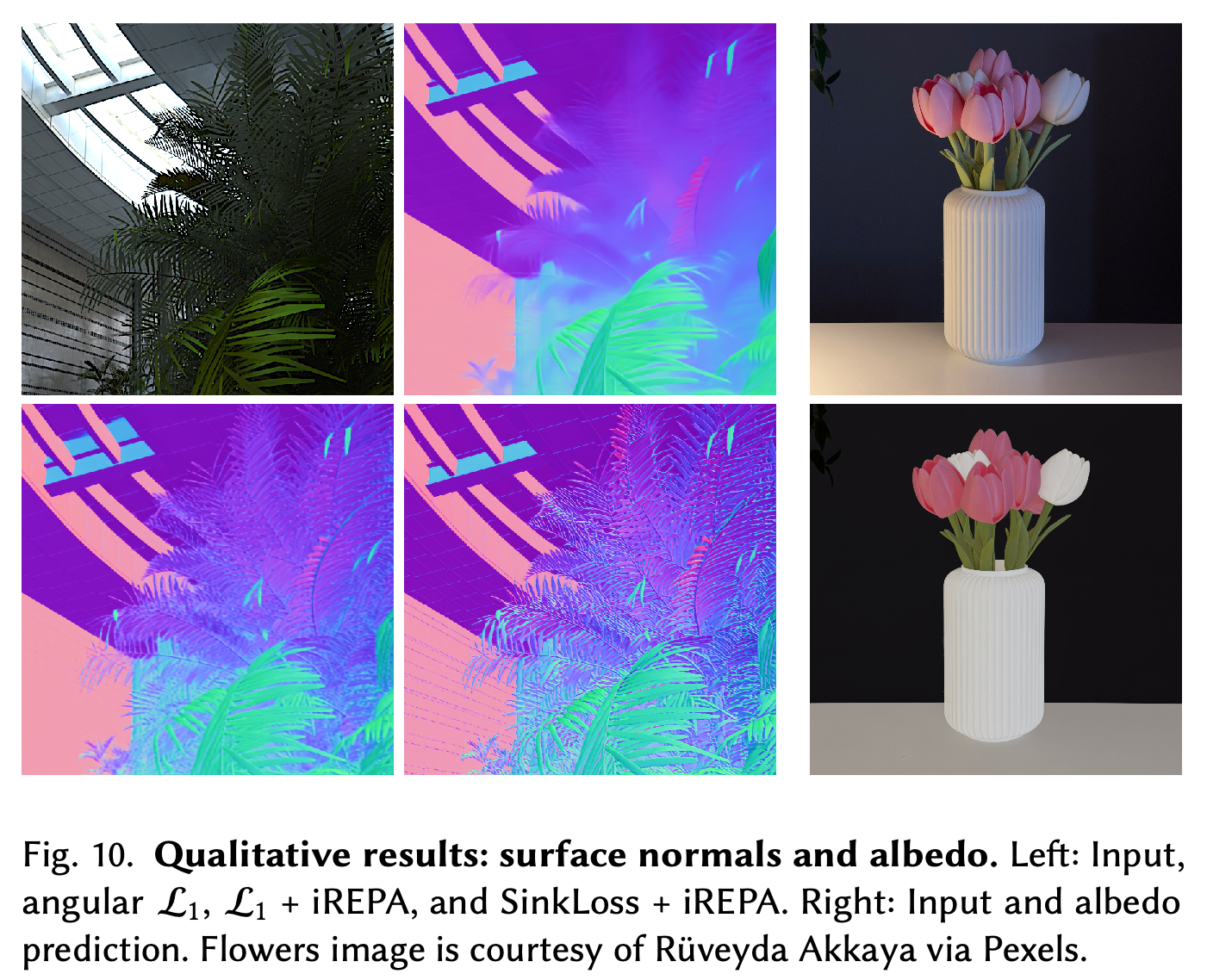
Compares in-the-wild depth, surface-normal, and albedo predictions. The figure provides qualitative evidence that the adapted model retains details such as hair, architectural lines, fur, and intrinsic-image structure across tasks.

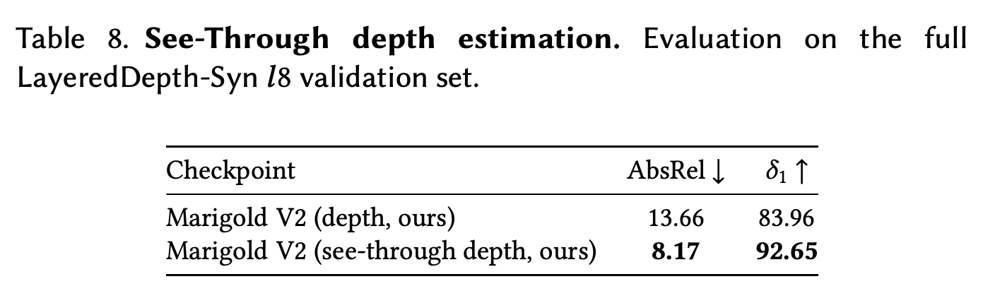
Shows that fine-tuning for the final LayeredDepth-Syn l8 layer improves see-through depth: AbsRel decreases from 13.66 to 8.17 and δ1 increases from 83.96 to 92.65.

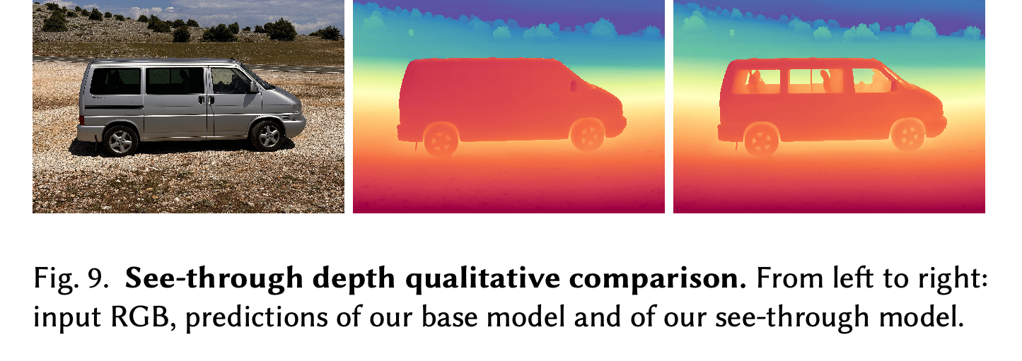
Contrasts input images with predictions from the base depth model and the see-through checkpoint. The specialized model is intended to estimate geometry behind transparent surfaces rather than the closer glass surface.

Illustrates normal-estimation variants using angular L1, L1 plus iREPA, and SinkLoss plus iREPA, alongside an albedo example. It visually supports transferring semantic alignment and local matching beyond depth.

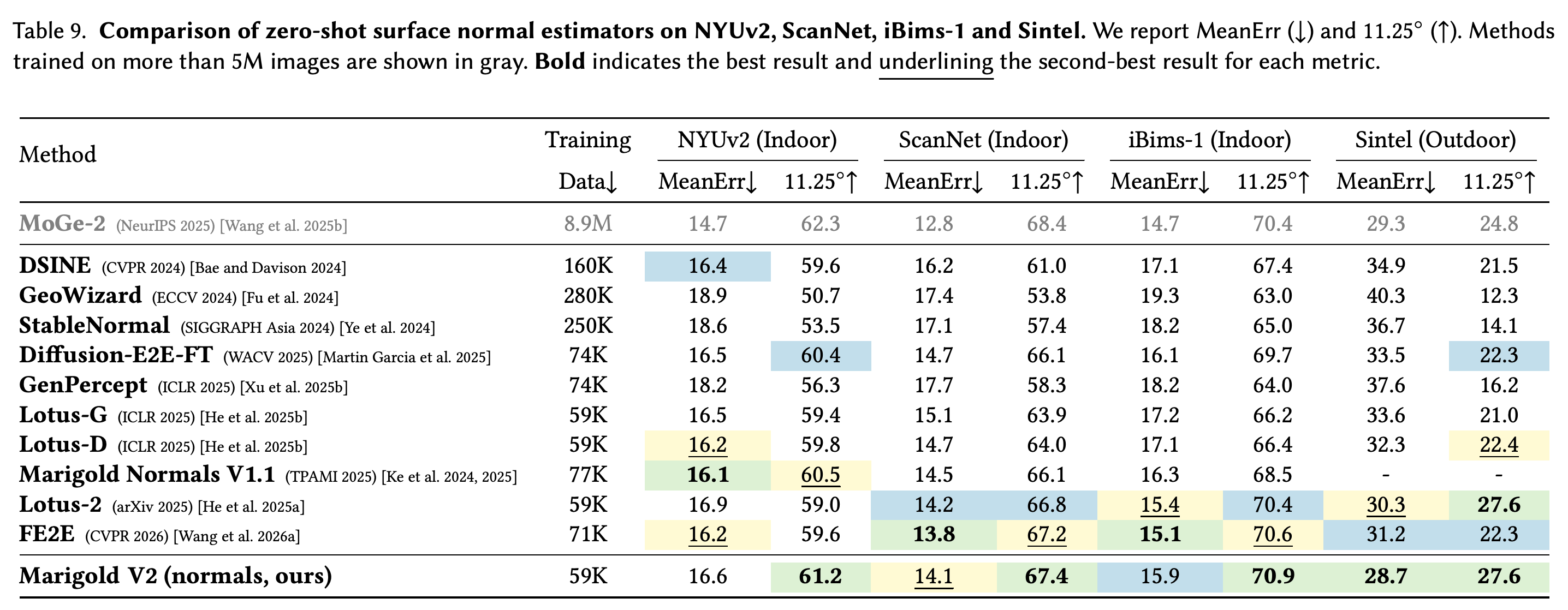
Compares zero-shot normal estimation over four datasets. Marigold V2 has the highest reported 11.25° rates on NYUv2, iBims-1, and Sintel, while its ScanNet result is close to the leading value but not the best.

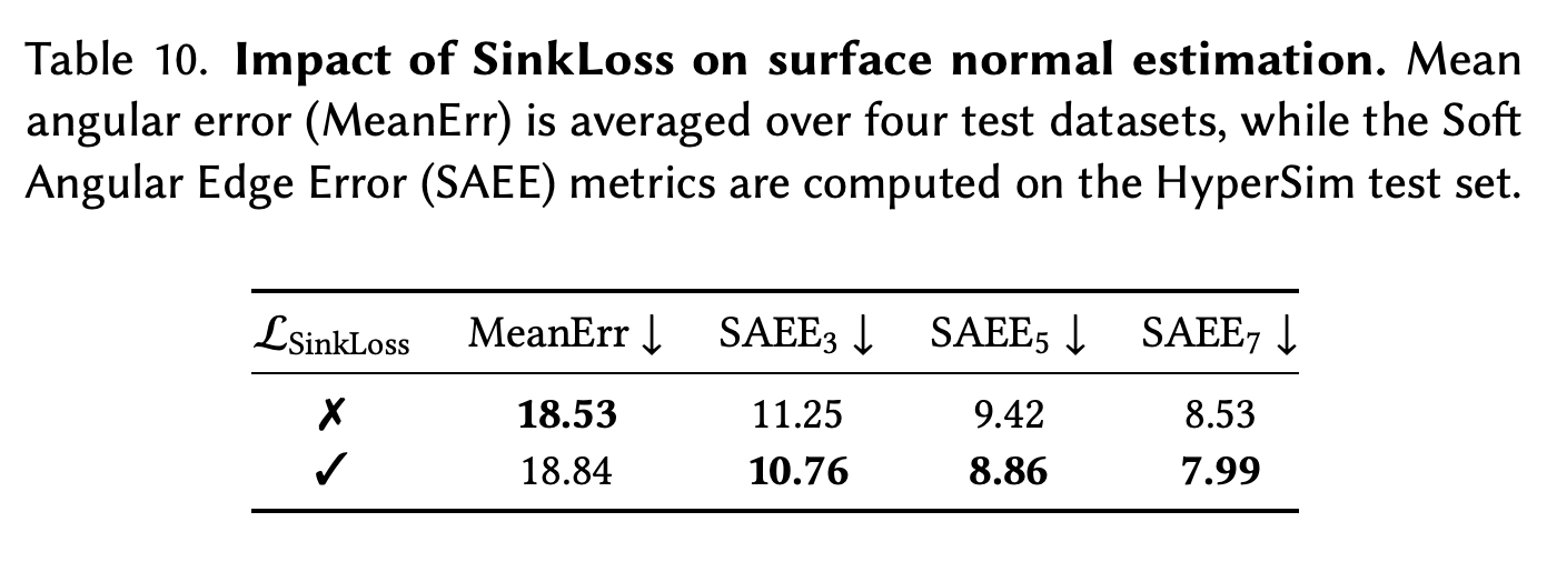
Shows the surface-normal trade-off from SinkLoss: average MeanErr rises from 18.53 to 18.84, while all boundary-specific SAEE metrics improve from 11.25/9.42/8.53 to 10.76/8.86/7.99.

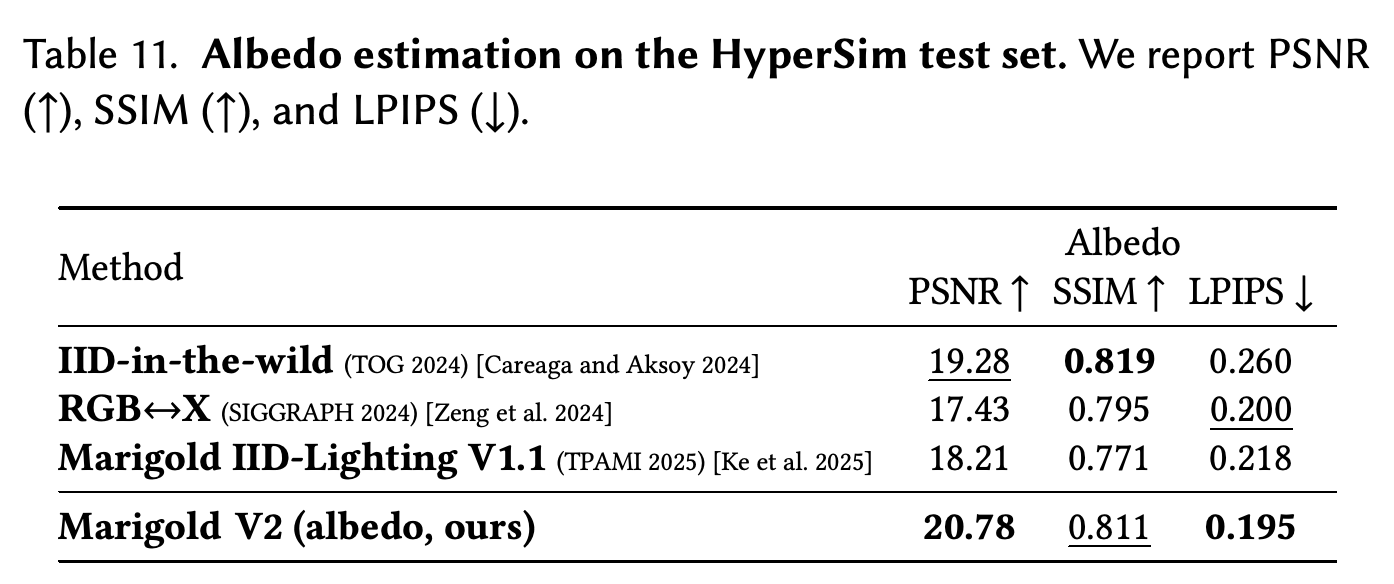
On HyperSim albedo estimation, Marigold V2 records the best reported PSNR of 20.78 and LPIPS of 0.195. Its SSIM of 0.811 is below IID-in-the-wild's 0.819.

5.1 Depth Completion

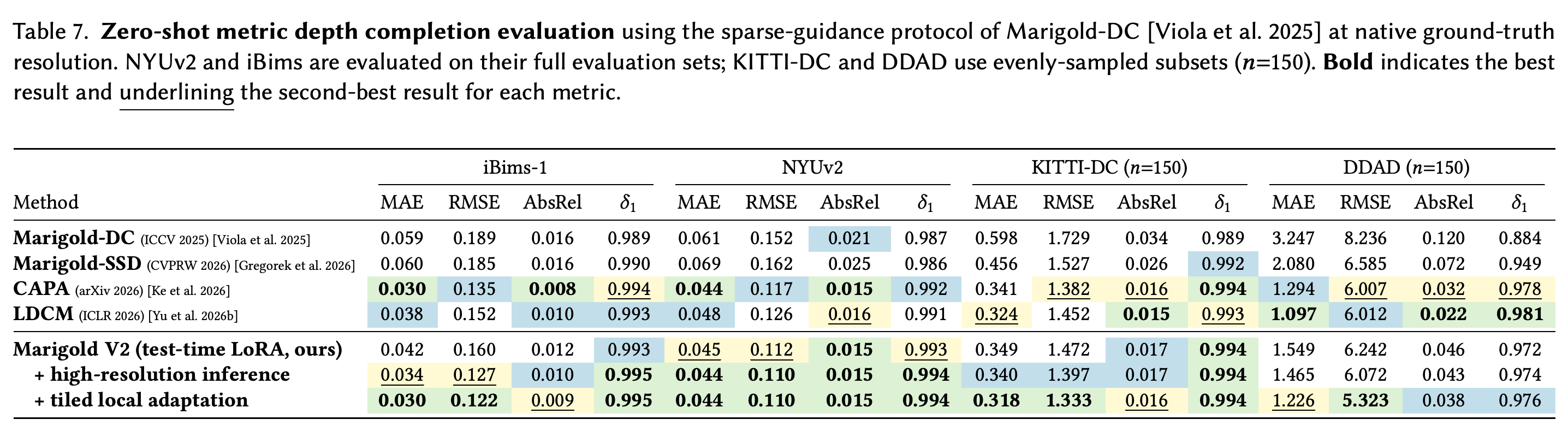
For metric depth completion, the method freezes the affine-invariant prior and optimizes a second rank-16 LoRA on the final 12 of 60 transformer blocks, together with scale and shift estimated from sparse measurements. With high-resolution inference and tiled local adaptation, it obtains RMSE of 0.122 on iBims-1, 0.110 on NYUv2, 1.333 on KITTI-DC, and 5.323 on DDAD, with tiling costing 4–14× the single-pass runtime.

Reports sparse-guided metric depth completion. The tiled local-adaptation variant has the lowest RMSE on all four listed benchmarks, including 0.122 on iBims-1 and 5.323 on DDAD.

Appendix

• The provided PDF has no separate appendix section. Its final pages contain References after the main-body conclusion.

Brief Thoughts

The central contribution is the explicit separation of aggregate depth accuracy from boundary fidelity: SinkLoss substantially improves Soft Edge Error while leaving average AbsRel nearly unchanged. The quantitative depth comparisons depend on RANSAC affine alignment and the paper’s comparable-training-data ranking rule, while the practical trade-off is high-resolution feasibility on one 32GB GPU rather than real-time inference.