Contrastive Learning, SimCLR 논문 설명(SimCLRv1, SimCLRv2)
09 Dec 2021 | Contrastive Learning Computer Vision SimCLR Google Research목차
- Contrastive Learning
- SimCLR(A Simple Framework for Contrastive Learning of Visual Representations)
- SimCLR v2(Big Self-Supervised Models are Strong Semi-Supervised Learners)
- References
이 글에서는 Contrastive Learning을 간략하게 정리한다.
Contrastive Learning
어떤 item들의 “차이”를 학습해서 그 rich representation을 학습하는 것을 말한다. 이 “차이”라는 것은 어떤 기준에 의해 정해진다.
Contrastive Learning은 Positive pair와 Negative pair로 구성된다. 단, Metric Learning과는 다르게 한 번에 3개가 아닌 2개의 point를 사용한다.
한 가지 예시는,
- 같은 image에 서로 다른 augmentation을 가한 다음
- 두 positive pair의 feature representation은 거리가 가까워지도록 학습을 하고
- 다른 image에 서로 다른 augmentation을 가한 뒤
- 두 negative pair의 feature representation은 거리가 멀어지도록 학습을 시키는
방법이 있다. 아래에서 간략히 소개할 SimCLR도 비슷한 방식이다.
Pair-wise Loss function을 사용하는데, 어떤 입력 쌍이 들어오면, ground truth distance $Y$는 두 입력이 비슷(similar)하면 0, 그렇지 않으면(dissmilar) 1의 값을 갖는다.
Loss function은 일반적으로 다음과 같이 나타낼 수 있다.
\[\mathcal{L}(W) = \sum^P_{i=1} L(W, (Y, \vec{X_1}, \vec{X_2})^i)\] \[L(W, (Y, \vec{X_1}, \vec{X_2})^i) = (1-Y)L_S(D^i_W) + YL_D(D^i_W)\]이때, 비슷한 경우와 그렇지 않은 경우 loss function을 다른 함수를 사용한다.
예를 들면,
\[L(W, (Y, \vec{X_1}, \vec{X_2})^i) = (1-Y)\frac{1}{2}(D_W)^2 + (Y)\frac{1}{2}( \max(0, m-D_W) )^2\]즉 similar한 경우 멀어질수록 loss가 커지고, dissimilar한 경우 가까워질수록 loss가 커진다.
SimCLR(A Simple Framework for Contrastive Learning of Visual Representations)
논문 링크: A Simple Framework for Contrastive Learning of Visual Representations
Github: https://github.com/google-research/simclr
- 2020년 2월(Arxiv), ICML
- Google Research
- Ting Chen, Simon Kornblith, Mohammad Norouzi, Geoffrey Hinton
Mini-batch에 $N$개의 image가 있다고 하면, 각각 다른 종류의 augmentation을 적용하여 $2N$개의 image를 생성한다. 이때 각 이미지에 대해, 나머지 $2N-1$개의 이미지 중 1개만 positive고 나머지 $2N-2$개의 image는 negative가 된다. 이렇게 하면 anchor에 대해 positive와 negative를 어렵지 않게 생성할 수 있고 따라서 contrastive learning을 수행할 수 있다.
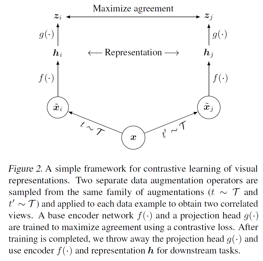
위의 그림을 보면.
- 이미지 $x$에
- 서로 다른 2개의 augmentation을 적용하여 $\tilde{x}_i, \tilde{x}_j$을 생성
- 이는 CNN 기반 network $f(\cdot)$를 통과하여 visual representation $h_i, $h_j$로 변환됨
- 이 표현을 projection head, 즉 MLP 기반 network인 $g(\cdot)$을 통과하여 $z_i, z_j$를 얻으면
- 이 $z_i, z_j$로 contrastive loss를 계산한다.
- 위에서 설명한 대로 mini-batch 안의 $N$개의 이미지에 대해 positive와 negative를 정해서 계산한다.
Contrastive loss는 다음과 같이 쓸 수 있다. (NT-Xent(Normalized Temperature-scaled Cross Entropy))
\[\ell_{(i, j)} = -\log \frac{\exp(\text{sim}(z_i, z_j) / \tau)}{\sum^{2N}_{k=1} \mathbb{1}_{[k \ne i]} \exp(\text{sim}(z_i, z_j) / \tau)}\]참고로 이는 self-supervised learning이다(사전에 얻은 label이 필요 없음을 알 수 있다).
Miscellaneous
- Projection head는 2개의 linear layer로 구성되어 있고, 그 사이에는 ReLU activation을 적용한다.
- Batch size가 클수록 많은 negative pair를 확보할 수 있으므로 클수록 좋다. SimCLR에서는 $N=4096$을 사용하였다.
- SGD나 Momemtum 등을 사용하지 않고 대규모 batch size를 사용할 때 좋다고 알려진 LARS optimizer를 사용하였다.
- Multi-device로 분산학습을 했는데, Batch Norm을 적용할 때는 device별로 따로 계산하지 않고 전체를 통합하여 평균/분산을 계산했다. 이러면 전체 device 간의 분포를 정규화하므로 정보 손실을 줄일 수 있다.
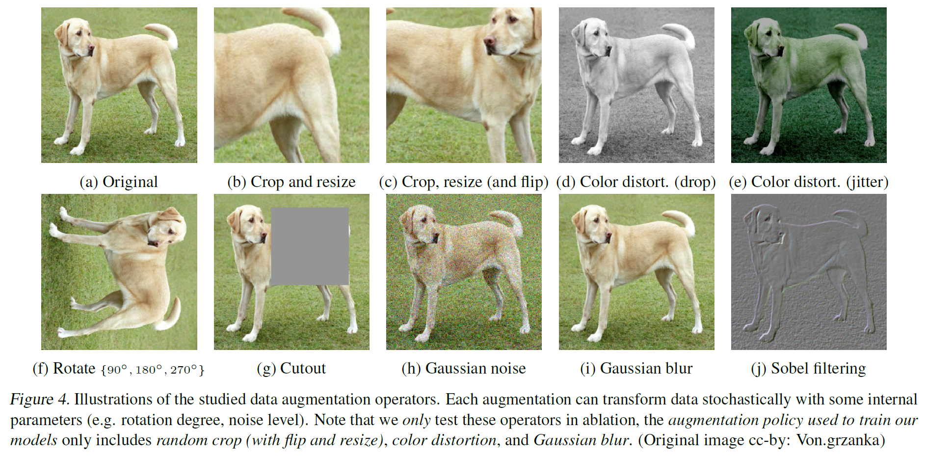
- Data Augmentation은
- Cropping/Resizing/Rotating/Cutout 등 이미지의 구도나 구조를 바꾸는 연산과
- Color Jittering, Color Droppinog, Gaussian Blurring, Soble filtering 등 이미지의 색깔을 변형하는 2가지 방식을 제안하였다.
- Augmentation 방법을 1개만 하는 것보다는 여러 개 하는 경우가 prediction task의 난이도를 높여 더 좋은 representation을 얻을 수 있다.
- 7가지의 data augmentation 방법 중 Random crop + Random Color Distortion 방식을 적용하면 가장 좋은 성능을 보인다고 한다.
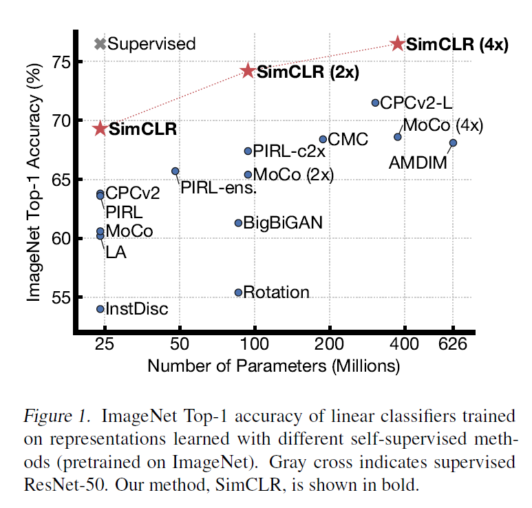
Experiments
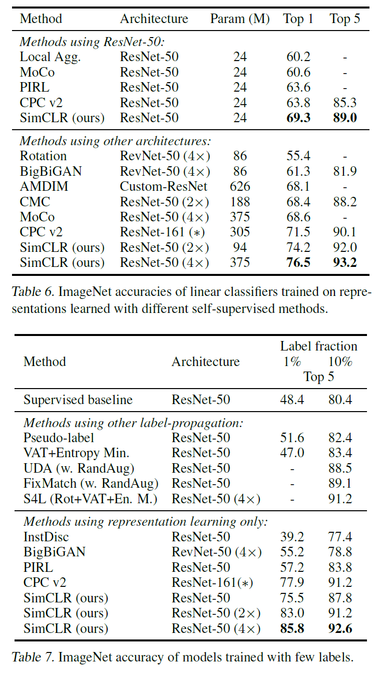
ImageNet에서 같은 모델 크기 대비 훨씬 좋은 성능을 보인다.
3가지 방법으로 평가한 결과는 아래 표에서 볼 수 있다.
- 학습된 모델을 고정하고 linear classifier를 추가한 linear evaluation
- 학습된 모델과 linear classifier를 모두 학습시킨 fine-tuning
- 학습된 모델을 다른 dataset에서 평가하는 transfer learning
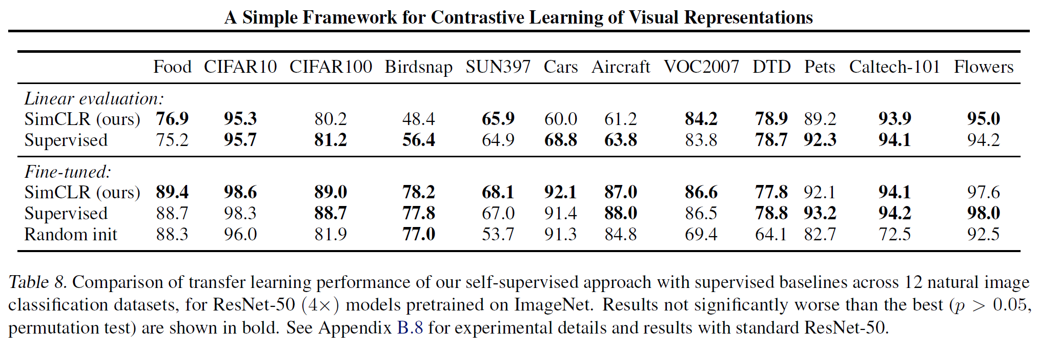
ImageNet 말고 다른 dataset에서 평가한 결과는 아래와 같다. Supervised 방식과 비등하거나 더 좋은 결과도 보여준다.
SimCLR v2(Big Self-Supervised Models are Strong Semi-Supervised Learners)
논문 링크: A Simple Framework for Contrastive Learning of Visual Representations
Github: https://github.com/google-research/simclr
- 2020년 6월(Arxiv), NIPS
- Google Research
- Ting Chen, Simon Kornblith, Kevin Swersky, Mohammad Norouzi, Geoffrey Hinton
SimCLR를 여러 방법으로 개선시킨 논문이며, computer vision에서 unsupervised learning 연구에 큰 기여를 했다.
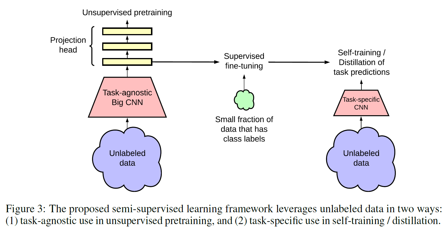
모델은 다음과 같은 과정을 따른다.
- Unsupervised(Self-supervised) Pre-training
- Supervised Fine-tuning
- Distillation using unlabeled data
이때 Unsupervsed 과정에서는 최종 task와는 무관한 데이터를 사용하였기에 task-agnostic이라는 용어를 사용한다.
Unsupervised(Self-supervised) Pre-training
대량의 unlabeled dataset으로 CNN model을 학습시켜 general representation을 모델이 학습하게 된다. SimCLR와 비슷하지만 다른 점은 SimCLRv1은 projection head를 버리고 downstream task를 수행하지만 v2는 1번째 head까지 포함시켜 fine-tuning이 시작된다.
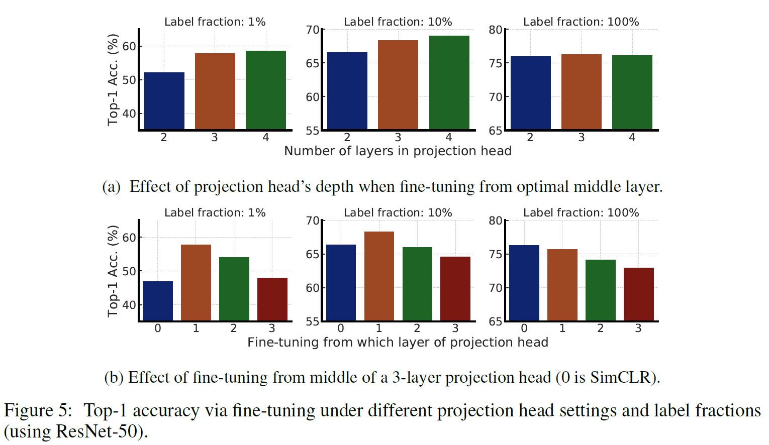
또한 Projection head의 linear layer 개수도 2개에서 3개로 늘었다.
그 이유는 label fraction(label이 되어 있는 비율)이 낮을수록 projection head의 layer가 더 많을수록 성능이 높아지기 때문이라고 한다.
Supervised Fine-tuning
전술했듯 Projection head의 1번째 layer까지 포함하여 fine-tuning을 진행한다.
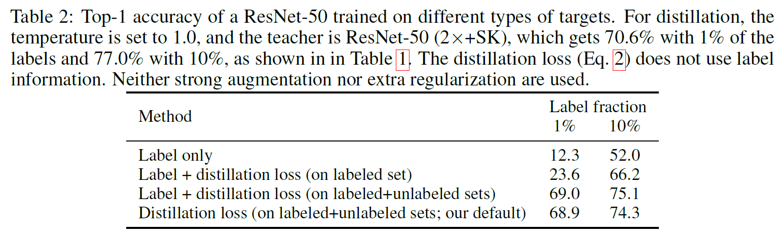
Distillation via unlaeled dataset
다음 과정을 통해 distillation을 수행한다.
- 학습시킬 모델은 student model이다.
- fine-tuning까지 학습된 teacher model을 준비한다. 이때 student model의 크기는 teacher보다 작다.
- Unlabeled data를 teacher model과 student model에 집어넣고 teacher model의 output distribution을 얻는다. 여기서 가장 높은 값의 pseudo-label을 얻고 이를 student model의 output distribution과 비교하여 loss를 minimize한다.
이 과정을 통해 teacher model이 갖고 있는 지식을 student model이 학습할 수 있게 된다. 그러면서 크기는 더 작기 때문에 효율적인 모델을 만들 수 있는 것이다.

Ground-truth label과 조합하여 가중합 loss를 계산할 수도 있다.

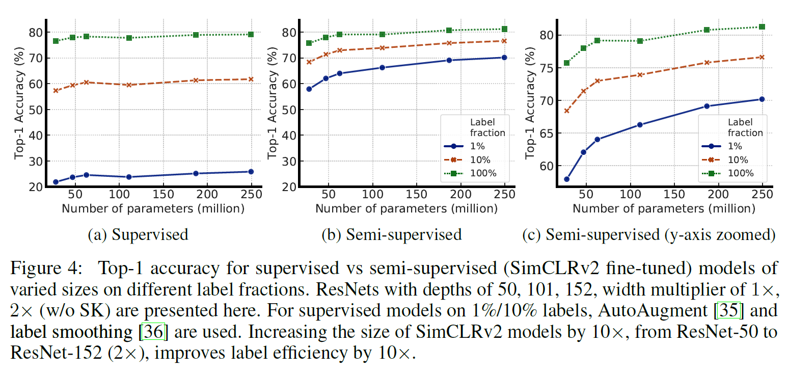
Experiments
더 큰 모델이 더 좋은 성능을 내는 건 어쩔 수 없는 것 같다..
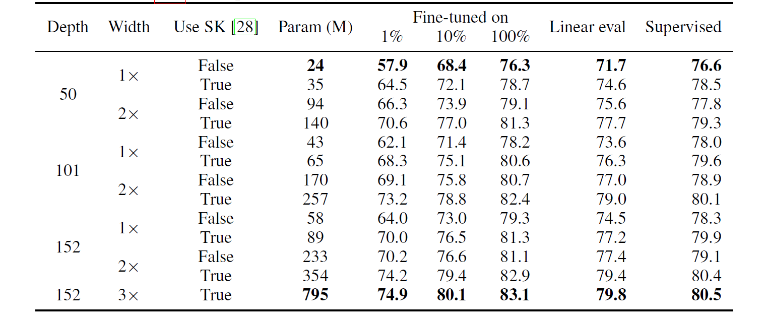
한 가지 눈여겨볼 것은 큰 모델일수록 label fraction이 낮은 dataset에 대해서 더 좋은 성능을 보인다는 것이다.
- 또 Projection head를 더 깊게 쌓거나 크기가 클수록 Representation을 학습하는 데 더 도움이 된다.
- Unlabeled data로 distillation을 수행하면 semi-supervised learning을 향상시킬 수 있다. 이때 label이 있는 경우 같이 사용해주면 좋은데, label이 있는 것와 없는 것을 따로 학습시키기보다는 distillation loss로 위에서 언급한 것처럼 가중합시킨 loss를 사용하면 성능이 가장 좋은 것을 확인할 수 있다.