mHC: Manifold-Constrained Hyper-Connections | Summary

Contents

Summary
1. Introduction
2. Related Works
- 2.1. Micro Design
- 2.2. Macro Design
3. Preliminary
- 3.1. Numerical Instability
- 3.2. System Overhead
4. Method
5. Experiments
6. Conclusion and Outlook
Appendix
Brief Thoughts

This article explains the key points of mHC: Manifold-Constrained Hyper-Connections.

2025-12-31 (arXiv)
Xie, Zhenda, Wei, Yixuan, Cao, Huanqi, Zhao, Chenggang, Deng, Chengqi, Li, Jiashi, Dai, Damai, Gao, Huazuo, Chang, Jiang, Yu, Kuai, et al.
DeepSeek-AI
Paper

Summary

mHC: Manifold-Constrained Hyper-Connections addresses the instability and memory-access overhead of Hyper-Connections (HC), which expand the residual stream and learn how its parallel streams interact. The paper identifies unconstrained products of residual mixing matrices as a source of signal amplification during large-scale language model pretraining.
mHC uses Sinkhorn-Knopp normalization to approximate doubly stochastic residual mappings; exact double stochasticity preserves stream averages while permitting information exchange. Fused mixed-precision kernels, selective recomputation, and an extended DualPipe schedule reduce the cost of the expanded stream, with the authors reporting 6.7% additional training time in in-house large-scale training at expansion rate n = 4.
On the 27B model, mHC reduces final training loss by 0.021 relative to the standard residual baseline, improves all eight downstream benchmarks, and exceeds HC on seven. Its measured composite backward propagation gain reaches approximately 1.6 rather than nearly 3000 for HC, although finite Sinkhorn-Knopp iterations leave approximation error and the published scaling experiments cover only 3B, 9B, and 27B models.

1. Introduction

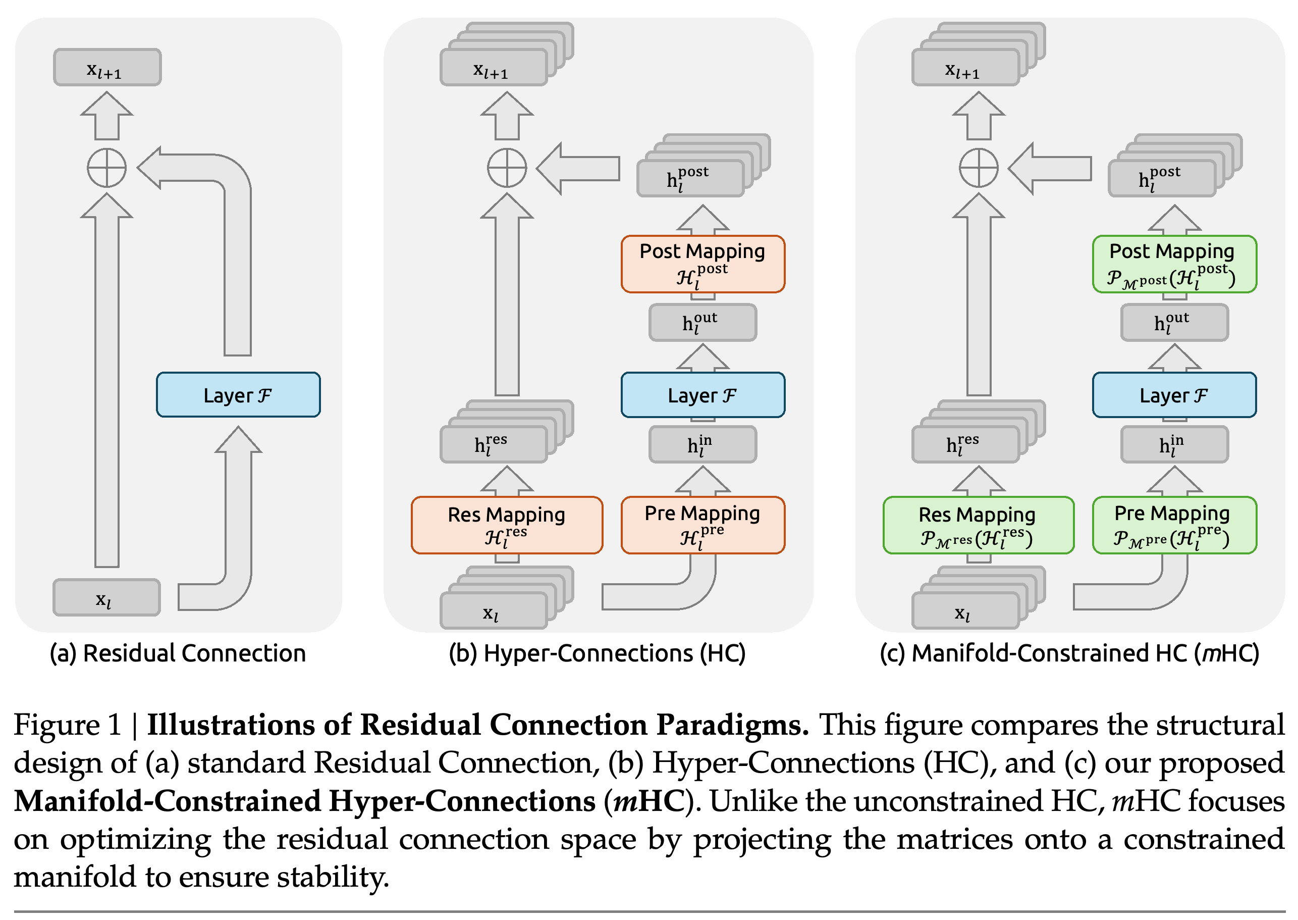
Standard residual connections propagate a representation through an unchanged additive path: (x_{l+1}=x_l+\mathcal{F}(x_l,W_l)). HC instead broadens the residual state from C to n × C and introduces learned pre-, post-, and residual mappings. Figure 1 shows that mHC retains this multi-stream topology but constrains its mappings, addressing cross-layer propagation stability and the hardware cost of the wider state.

The pre-mapping aggregates n streams into the C-dimensional input of F; the post-mapping distributes its output back to the streams; the residual mapping mixes the streams directly.
Across depth, HC replaces the unchanged residual path with a product of learned residual matrices. Unconstrained products can amplify or attenuate signals, whereas exactly doubly stochastic products conserve the mean across streams.

Standard residual connections, Hyper-Connections, and Manifold-Constrained Hyper-Connections, showing their residual, pre-, and post-mapping structures.

The related-work discussion separates micro-design, which determines computations inside a block, from macro-design, which determines how representations are propagated, routed, and merged between blocks. mHC primarily changes macro-design rather than the attention or feed-forward computation itself.

2.1. Micro Design

The micro-design review traces the transition from convolutional blocks to attention and Feed-Forward Networks (FFNs). It discusses Multi-Query Attention (MQA), Grouped-Query Attention (GQA), and Multi-Head Latent Attention (MLA) as efficiency-oriented attention variants, and Mixture-of-Experts (MoE) as a way to increase parameter capacity without proportional active computation.

2.2. Macro Design

The macro-design review connects ResNet, DenseNet, FractalNet, and Deep Layer Aggregation to more recent attempts to expand residual capacity. HC learns connection strengths, Residual Matrix Transformer stores features in an outer-product memory matrix, and MUDDFormer uses multiway dynamic dense connections. The paper positions mHC as an HC extension that constrains stream mixing and explicitly addresses memory traffic.

3. Preliminary

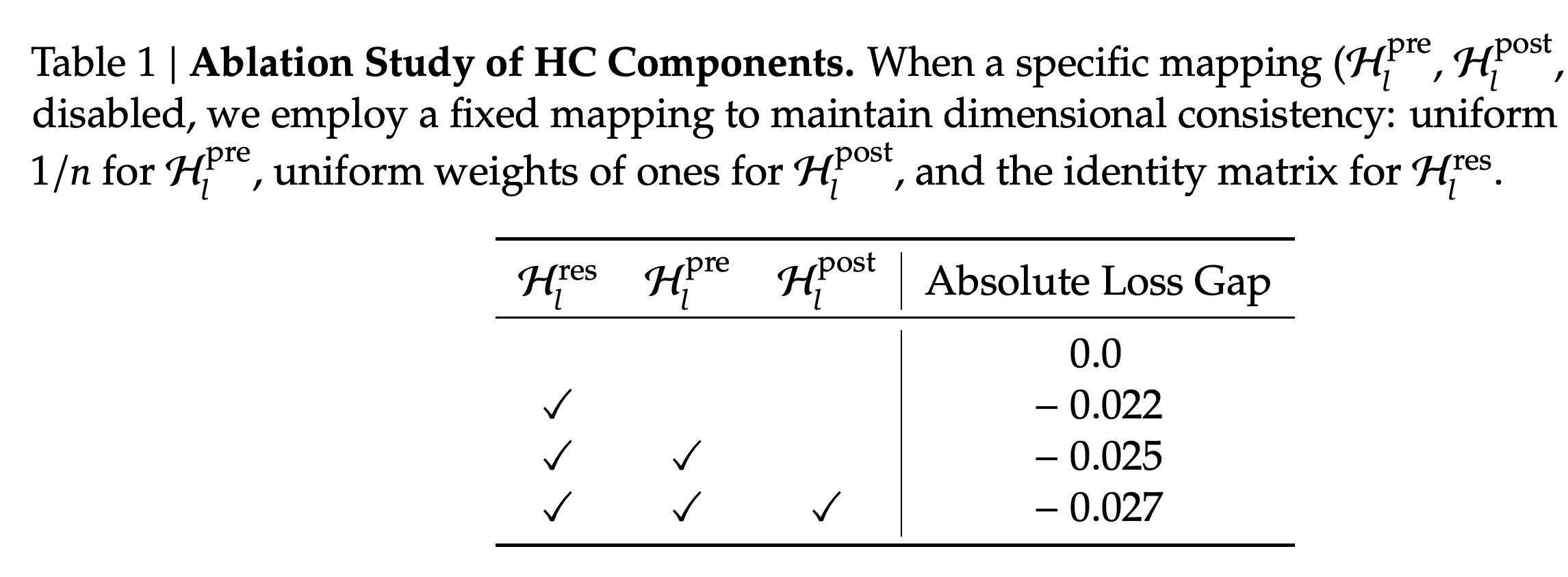
HC represents the residual state as an n × C matrix and learns input-dependent dynamic coefficients together with global static coefficients. Its propagation rule is x_{l+1} = H_l^{res}x_l + (H_l^{post})^T F(H_l^{pre}x_l, W_l). Table 1 indicates that learning residual-stream mixing accounts for most of the measured loss improvement in the component ablation.

Original HC derives dynamic coefficients from RMSNorm-normalized features, linear projections, tanh, and small initialized learnable gates, then adds learnable static biases.
The ablation reports loss gaps of 0.0 with all mappings fixed, −0.022 with only the residual mapping learned, −0.025 after also learning the pre-mapping, and −0.027 with all three learned.
Disabled mappings use uniform pre-weights of 1/n, post-weights of one, and an identity residual matrix. These fixed mappings preserve dimensional consistency while isolating the contribution of learned mappings.

HC component ablation with fixed dimension-preserving mappings used when a learnable component is disabled.

3.1. Numerical Instability

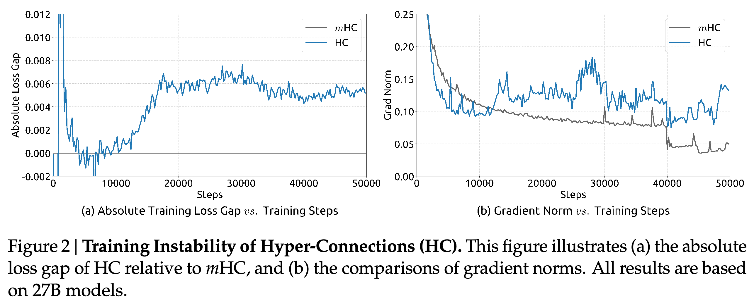
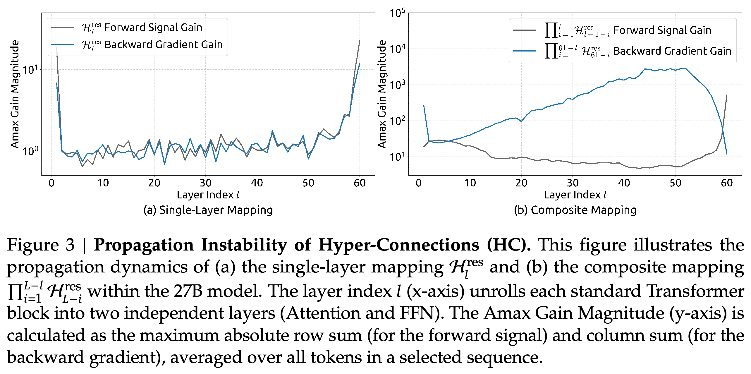
The 27B HC run exhibits a loss surge around step 12k accompanied by unstable gradient norms, as shown in Figure 2. Figure 3 links this behavior to accumulated residual mappings: composite backward Amax Gain Magnitude peaks near 3000 even though many individual mappings have gains near one.

Forward Amax Gain Magnitude is the maximum absolute value of the residual mapping’s row sums; backward gain uses its column sums. These are signed sums before taking absolute values, not sums of absolute entries, and the plotted measurements are averaged over tokens in a selected sequence.
The layer axis treats attention and FFN as separate residual layers, yielding 60 residual layers for the 30-block 27B model.
These measurements diagnose amplification in the residual mixing path. For signed HC matrices, they are not general induced-norm bounds, and they do not measure the full network Jacobian.

Training-loss gap relative to mHC and gradient-norm trajectories for 27B HC and mHC models.

Single-layer and composite HC residual propagation gains across attention and FFN residual layers in the 27B model.

3.2. System Overhead

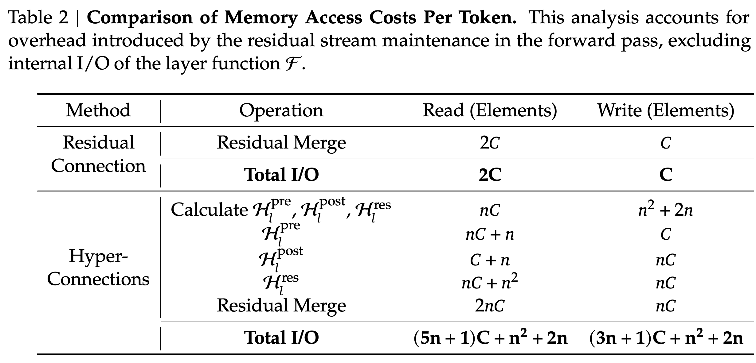
Low additional FLOPs do not imply low runtime overhead for HC. Table 2 shows that maintaining the expanded stream increases forward memory traffic roughly in proportion to n, while learned mappings also require additional backward activations and pipeline parallelism communicates an n-fold wider residual state.

Excluding internal I/O of F, a standard residual merge reads 2C elements and writes C elements per token.
The unfused HC accounting reads (5n + 1)C + n² + 2n elements and writes (3n + 1)C + n² + 2n elements per token.
The resulting bandwidth demand, activation memory, and pipeline communication motivate fusion, recomputation, and communication-computation overlap.

Per-token forward memory-access costs of standard residual connections and HC, excluding internal I/O of the layer function.

4. Method

The method combines constrained residual-stream mappings with infrastructure optimizations. The constraint controls mixing across depth without fixing the residual matrix to the identity, which would eliminate information exchange between streams.

4.1. Manifold-Constrained Hyper-Connections

mHC restricts the residual mapping to the Birkhoff polytope: H_l^{res}1_n = 1_n, 1_n^T H_l^{res} = 1_n^T, and H_l^{res} ≥ 0. Each output stream is therefore a convex combination of input streams, and the average across streams is conserved under an exact constraint.

An exactly doubly stochastic matrix has spectral norm at most one, making the residual mixing operation non-expansive. This is a norm bound, not preservation of every input vector’s norm.
Doubly stochastic matrices are closed under multiplication, so exact residual mappings retain their conservation property when composed across depth.
The Birkhoff polytope is the convex hull of permutation matrices, providing an interpretation as mixtures of stream permutations. At n = 1, the residual mapping reduces to the scalar one.
mHC additionally makes pre- and post-mapping coefficients non-negative to avoid cancellation caused by signed aggregation and redistribution.

4.2. Parameterization and Manifold Projection

mHC flattens the full n × C residual state before RMSNorm and dynamic coefficient prediction, allowing each mapping to depend on all streams. It applies sigmoid to the pre-mapping logits, twice sigmoid to the post-mapping logits, and Sinkhorn-Knopp normalization to the residual logits.

The dynamic projection dimensions are nC × n for pre- and post-mappings and nC × n² for the residual mapping. Learnable gates and static biases are then applied.
Sinkhorn-Knopp starts from M^(0) = exp(H̃_l^{res}) and iterates (M^{(t)}=\mathcal{T}_r\left(\mathcal{T}_c\left(M^{(t-1)}\right)\right)), where T_c and T_r normalize columns and rows, respectively.
The exact doubly stochastic limit requires convergence. The experiments use t_max = 20, trading normalization accuracy against computational cost.

4.3. Efficient Infrastructure Design

4.3.1. Kernel Fusion reduces bandwidth and launch overhead by combining coefficient calculations and mapping applications. The implementation moves division by the RMS norm after the projection, absorbs the RMSNorm weight into the projection parameters, and uses mixed precision for coefficient calculation.

The input state is bfloat16, the consolidated projection is tfloat32, and gates, biases, and coefficient outputs are float32. Projection and norm calculations share a fused kernel; small coefficient transformations use another kernel.
Sinkhorn-Knopp iterations run inside one kernel. A custom backward kernel recomputes intermediate normalization results on-chip.
Fusing post-mapping, residual mixing, and residual merge reduces reads for that application kernel from (3n + 1)C to (n + 1)C and writes from 3nC to nC.
Most kernels, excluding the projection-and-norm kernels corresponding to Eq. (14)–(15), are implemented using TileLang.

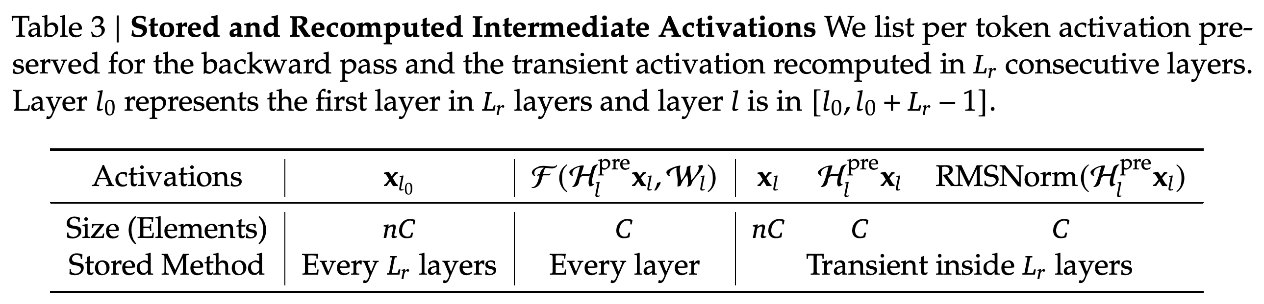
4.3.2. Recomputing discards intermediate mHC activations after the forward pass and reconstructs them during backpropagation without rerunning the expensive layer function F. Table 3 distinguishes persistent block inputs and layer outputs from transient reconstructed states.

For each block of L_r residual layers, the implementation retains the nC-element initial residual state; each layer’s C-element output of F is also retained.
The block-size-dependent memory objective is nC⌈L/L_r⌉ + (n + 2)CL_r, giving the approximate optimum L_r* ≈ √(nL/(n + 2)).
Recomputation blocks cannot cross pipeline-stage boundaries. The implementation aligns them with stages because the theoretical optimum typically lies near the stage depth.

Stored and transiently recomputed per-token activations within a block of consecutive residual layers.

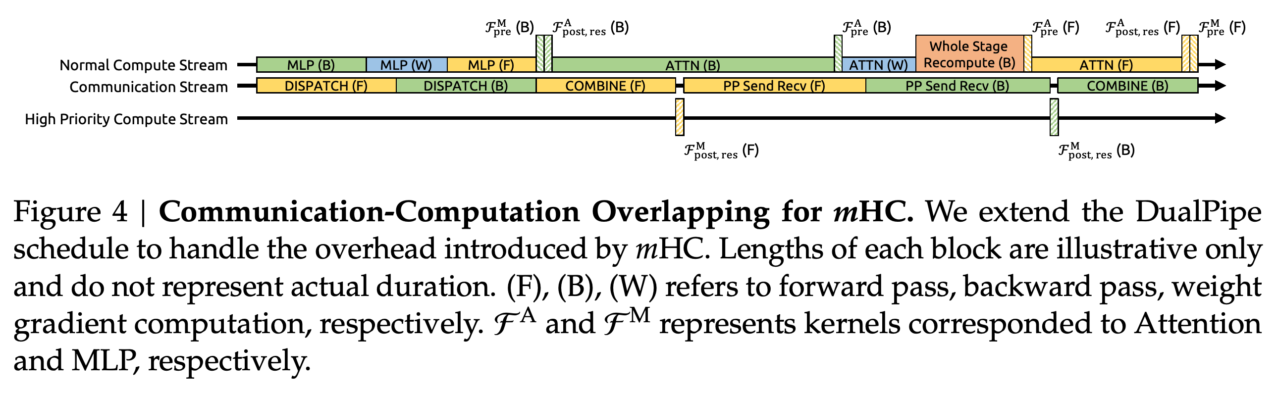
4.3.3. Overlapping Communication in DualPipe extends the pipeline schedule to overlap widened-state communication and stage-level recomputation with other work. Figure 4 illustrates the coordination of normal computation, communication, and a high-priority compute stream; its block lengths are schematic rather than measured timings.

FFN post-mapping and residual-merge kernels execute on the high-priority stream so that pipeline communication is not blocked behind longer computations.
Long-running attention operations avoid persistent kernels, allowing more flexible scheduling of overlapping work.
Recomputation can proceed independently of pipeline communication because the initial residual state of each stage is already cached locally. The authors report 6.7% additional training time at n = 4 with the combined infrastructure design.

Extended DualPipe communication-computation overlap using normal compute, communication, and high-priority compute streams.

5. Experiments

The experiments evaluate language model pretraining through convergence, downstream benchmark performance, scaling behavior, and residual propagation diagnostics. The principal comparisons are the standard residual baseline, HC, and mHC.

5.1. Experimental Setup

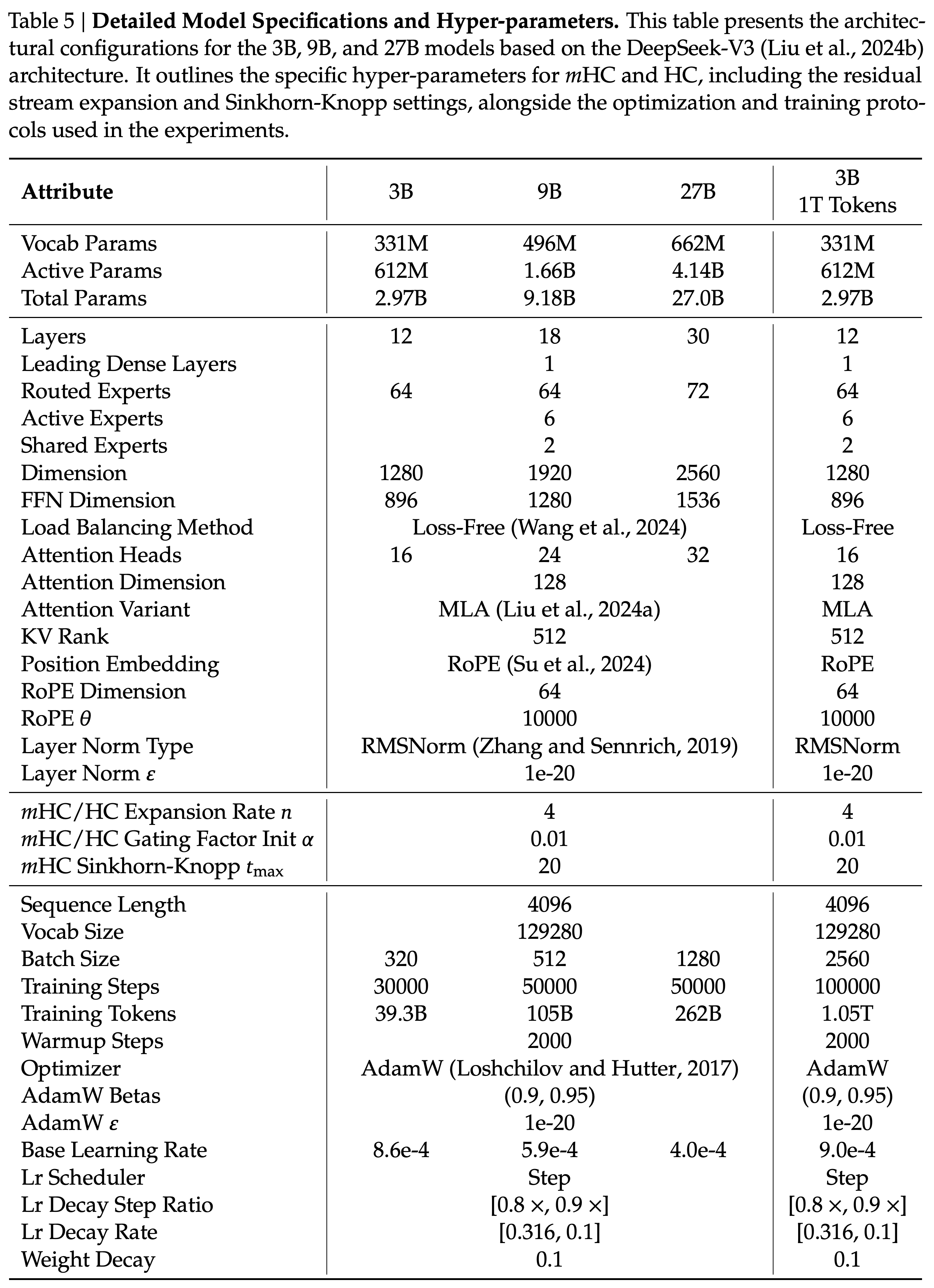
The models use MoE architectures inspired by DeepSeek-V3, with n = 4 for both HC and mHC. Compute-scaling experiments use 3B, 9B, and 27B models trained on proportionally sized datasets; a separate 3B run examines token scaling with a corpus described as 1 trillion tokens, with Table 5 reporting 1.05T training tokens.

The nominal 3B, 9B, and 27B models have 2.97B, 9.18B, and 27.0B total parameters, respectively, but 612M, 1.66B, and 4.14B active parameters.
Their training budgets are 39.3B, 105B, and 262B tokens over 30000, 50000, and 50000 steps. All configurations use sequence length 4096.
Table 5 specifies architecture and optimization settings, including 12, 18, and 30 Transformer blocks and 20 Sinkhorn-Knopp iterations.

Architecture specifications, HC and mHC settings, and optimization hyperparameters for the three model scales and the extended 3B training run.

5.2. Main Results

For the 27B models, Figure 5 shows that mHC avoids the sustained loss deterioration observed in HC and finishes with a 0.021 loss reduction relative to the baseline. Its gradient-norm trajectory is steadier than HC’s and approaches the baseline’s profile later in training.

Baseline-relative training-loss gaps and gradient norms for the 27B baseline, HC, and mHC runs.

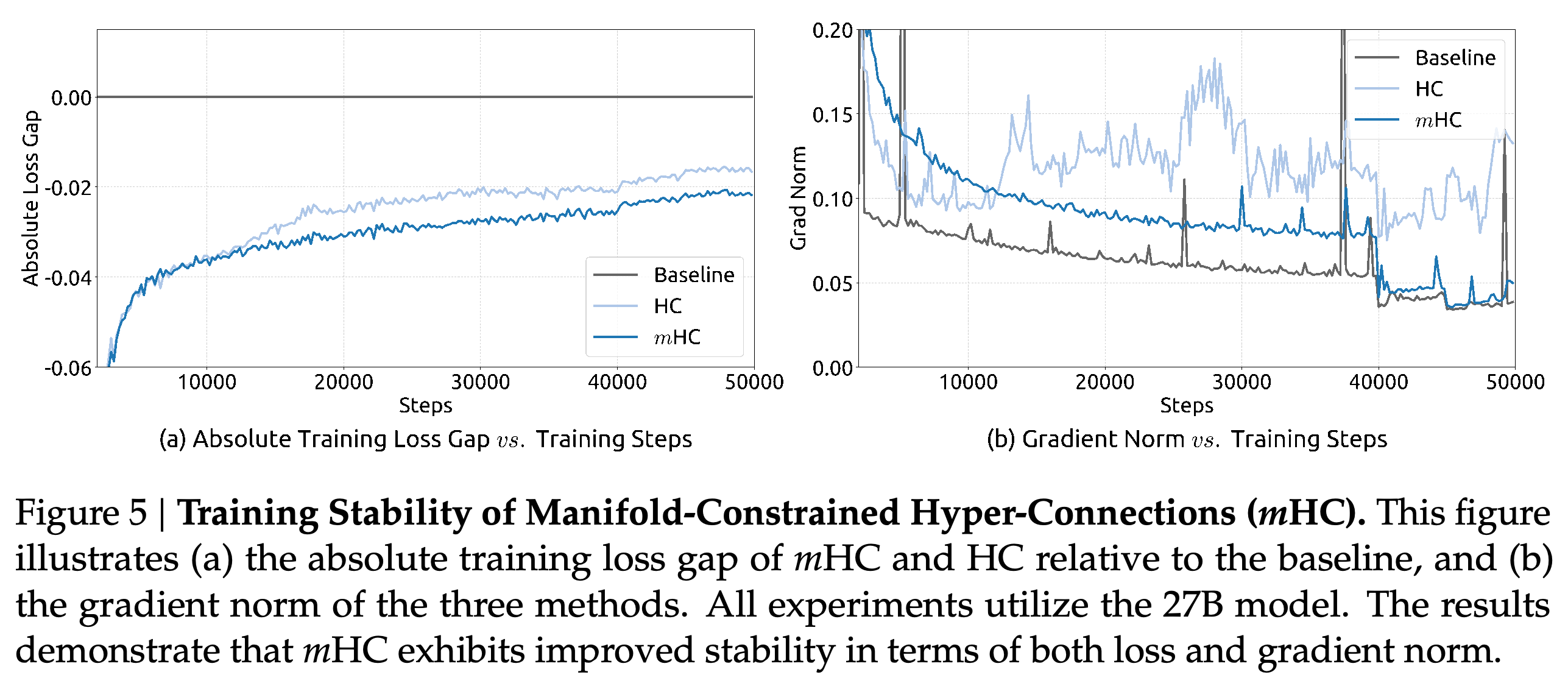
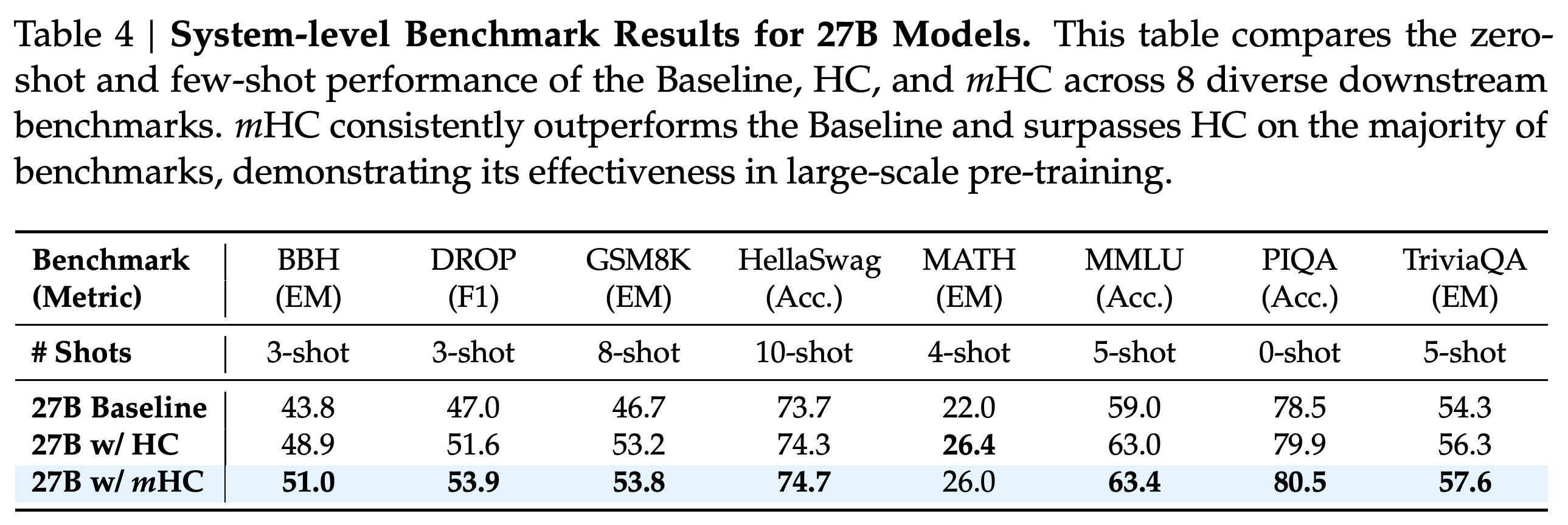
Table 4 shows that mHC improves every evaluated downstream benchmark over the baseline and seven of eight over HC. Relative to HC, BBH increases from 48.9 to 51.0 and DROP from 51.6 to 53.9; MATH is the exception, falling from 26.4 to 26.0 while remaining above the baseline’s 22.0.

The evaluation uses BBH 3-shot EM, DROP 3-shot F1, GSM8K 8-shot EM, HellaSwag 10-shot accuracy, MATH 4-shot EM, MMLU 5-shot accuracy, PIQA 0-shot accuracy, and TriviaQA 5-shot EM.
In that benchmark order, baseline scores are 43.8, 47.0, 46.7, 73.7, 22.0, 59.0, 78.5, and 54.3; HC scores are 48.9, 51.6, 53.2, 74.3, 26.4, 63.0, 79.9, and 56.3.
mHC scores are 51.0, 53.9, 53.8, 74.7, 26.0, 63.4, 80.5, and 57.6. The BBH and DROP differences are 2.1 and 2.3 percentage points on the reported score scales.

Zero-shot and few-shot downstream benchmark results for 27B baseline, HC, and mHC models, including metrics and shot counts.

5.3. Scaling Experiments

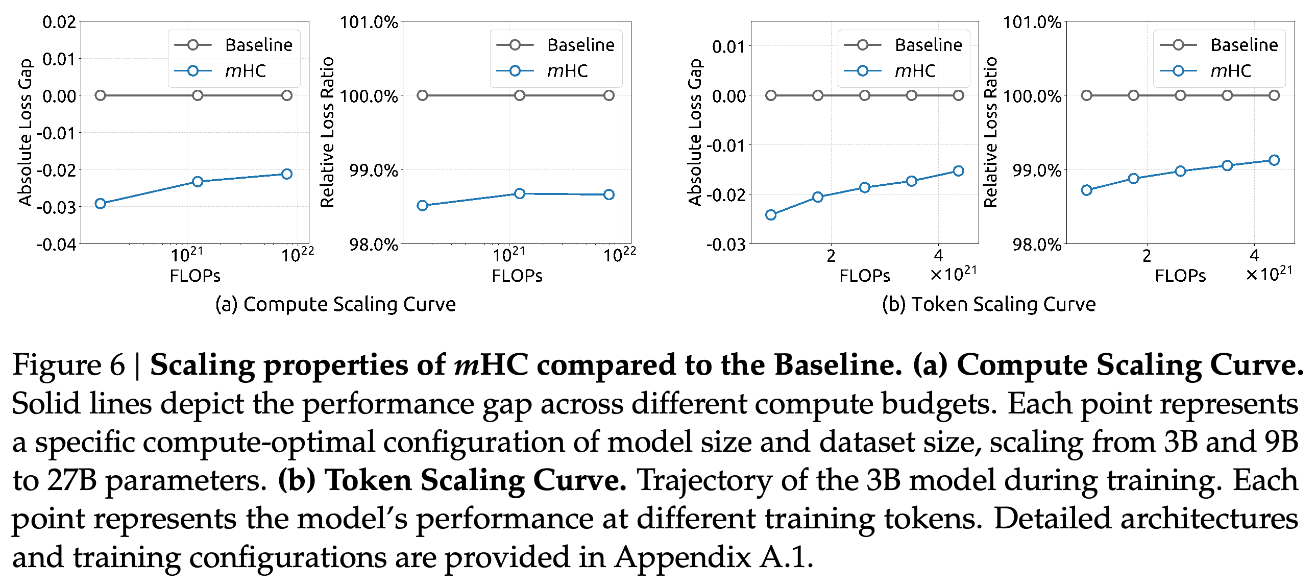
Figure 6 shows that mHC’s loss advantage over the baseline persists across the 3B, 9B, and 27B compute-scaling configurations, with some attenuation at larger budgets. The separate 3B token-scaling trajectory also retains an advantage as training progresses, although the gap narrows.

Compute scaling changes both model size and training-data size; token scaling follows checkpoints within one 3B training run.
The plots report both absolute loss gaps and relative loss ratios. They support a persistent benefit within the tested budgets, not unrestricted extrapolation to larger scales.
The authors additionally cite in-house large-scale training, but do not provide its model configurations or detailed results in the PDF.

Compute-scaling loss comparisons across 3B, 9B, and 27B models and token-scaling comparisons within the separate 3B run.

5.4. Stability Analysis

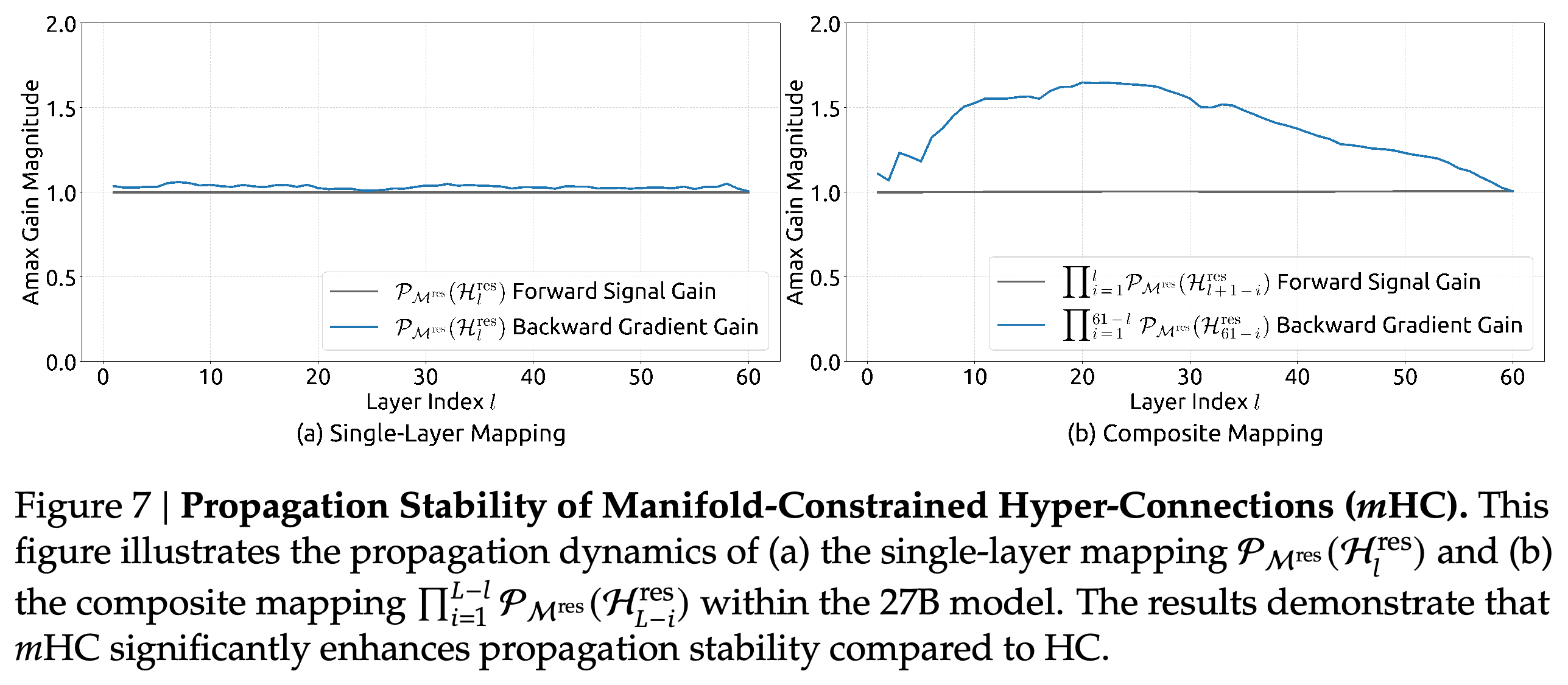
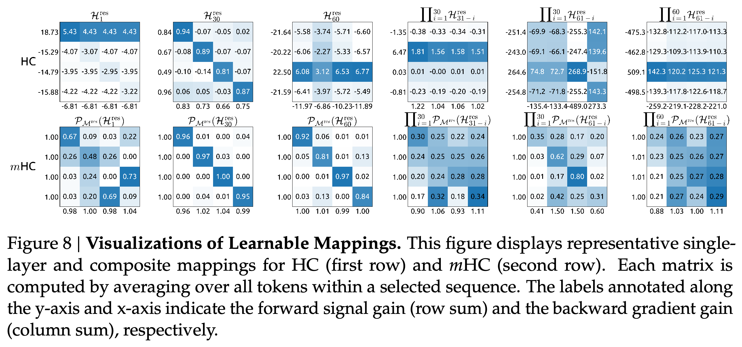
Figure 7 shows forward residual gain near one and small single-layer backward deviations associated with the finite 20-iteration Sinkhorn-Knopp approximation. Across composed mappings, backward gain reaches approximately 1.6, compared with nearly 3000 for HC. Figure 8’s representative matrices show large signed coefficients in HC and non-negative coefficients with much smaller row- and column-sum deviations in mHC.

The last row-normalization operation keeps row sums close to one, while column sums can retain approximation error; those errors can accumulate under composition.
The reported reduction is approximately three orders of magnitude in this residual-path diagnostic.
The matrix visualizations and gain curves use a selected sequence, so they illustrate the mechanism rather than establish a worst-case bound over all model inputs.

Single-layer and composite residual propagation gains for mHC in the 27B model.

Representative token-averaged single-layer and composite residual matrices for HC and mHC, annotated with row and column gains.

6. Conclusion and Outlook

The conclusion attributes mHC’s benefit to controlled multi-stream mixing that retains HC’s representational flexibility while reducing propagation instability. Its practical contribution also includes the implementation needed to limit the wider residual state’s training overhead. Alternative geometric constraints are proposed as future work, rather than demonstrated in the experiments.

Appendix

A.1. Detailed Model Specifications and Hyper-parameters. Table 5 reports model widths of 1280, 1920, and 2560 and FFN dimensions of 896, 1280, and 1536 for the 3B, 9B, and 27B configurations. They use 64, 64, and 72 routed experts, six active experts, two shared experts, one leading dense layer, MLA with KV rank 512, and loss-free load balancing. Common settings include RoPE dimension 64, RoPE θ = 10000, RMSNorm ε = 1e-20, vocabulary size 129280, residual expansion 4, gating initialization 0.01, and 20 Sinkhorn-Knopp iterations.
In the order 3B, 9B, 27B, and extended 3B, the four configurations use batch sizes 320, 512, 1280, and 2560; training steps 30000, 50000, 50000, and 100000; and base learning rates 8.6e-4, 5.9e-4, 4.0e-4, and 9.0e-4. AdamW uses betas (0.9, 0.95), ε = 1e-20, weight decay 0.1, and 2000 warmup steps. The step scheduler specifies decay step ratios [0.8 ×, 0.9 ×] and decay rates [0.316, 0.1].

Brief Thoughts

The propagation diagnostics and training outcomes provide complementary evidence: constrained matrices reduce the measured residual gain, the 27B run remains steadier, and downstream performance generally improves. The systems analysis is useful because it distinguishes low additional FLOPs from substantial memory traffic and communication costs.

The phrase “restore the identity mapping property” describes conservation and non-expansiveness of the exactly constrained residual mixing path, not an identity transformation of every representation. Exact doubly stochastic mixing can still contract stream differences, and the analysis does not establish global stability for input-dependent mappings and the full nonlinear network. The PDF also lacks multi-seed uncertainty estimates, expansion-rate and iteration-count sweeps, and a hardware-specific timing breakdown needed to assess the portability of the reported 6.7% overhead.