Tapered Language Models | Summary

Contents

Summary
1. Introduction
2. Tapered Language Models
3. Experiments
4. Layer-wise Novelty
5. Related Work
6. Limitations
7. Discussion and Conclusion
Appendix
Brief Thoughts

This article explains the key points of Tapered Language Models.

2026-06-22 (arXiv)
Bayat, Reza, Behrouz, Ali, Courville, Aaron.
Mila, Cornell University, Université de Montréal, CIFAR AI Chair
Paper

Summary

Tapered Language Models tests whether language models should allocate equal parameter capacity to every layer. The proposed intervention monotonically decreases MLP intermediate width across depth while preserving its average, leaving total parameters and training and inference FLOPs unchanged.
A 15-configuration sweep on a 440M Transformer selects a cosine taper from 1.50 to 0.50 times the baseline MLP width, reducing in-distribution validation perplexity from 16.28 to 14.44. Transferring this configuration unchanged to four architectures at 760M and 1.3B improves average commonsense accuracy in all eight comparisons, LAMBADA perplexity in all eight, and WikiText perplexity in seven.
Measurements on pretrained GPT-2 models show that later MLP updates become more aligned with the incoming residual stream, providing observational support for allocating more capacity earlier. The paper does not establish a causal mechanism, optimal profiles across architectures and scales, measured runtime savings, or applicability to other architectural dimensions.

1. Introduction

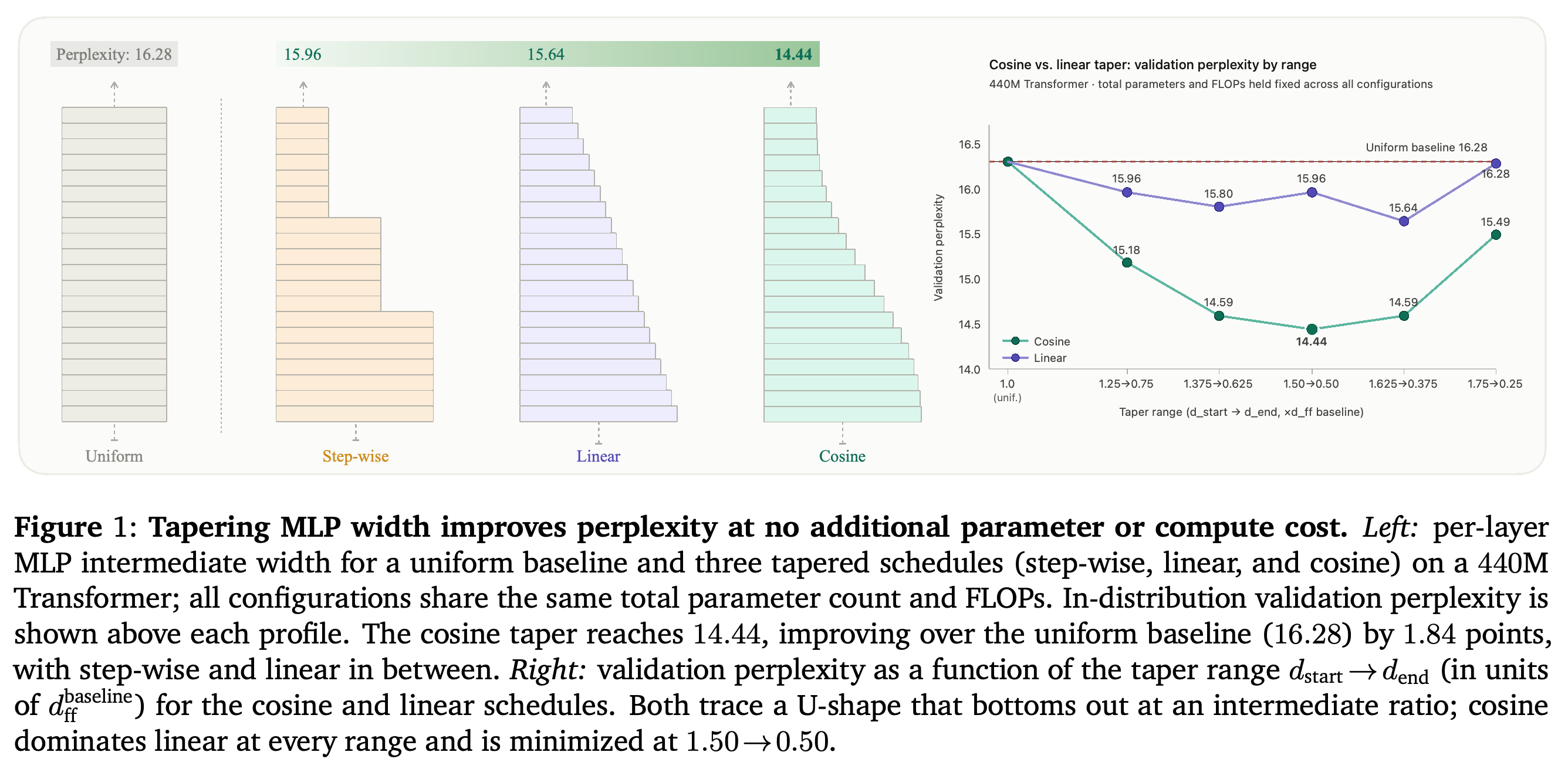
Transformer, recurrent, and memory-based language models commonly pair a token-mixing module with an MLP in each layer and distribute capacity uniformly across depth. The paper challenges this default using prior evidence from early exit, layer skipping, redundancy analysis, and interpretability that layer contributions differ with depth. Figure 1 previews how smooth width reallocation can improve perplexity without enlarging the model or its FLOP budget.

Equal-budget MLP width profiles and validation perplexity for a 440M Transformer, with cosine and linear results across five taper ranges.

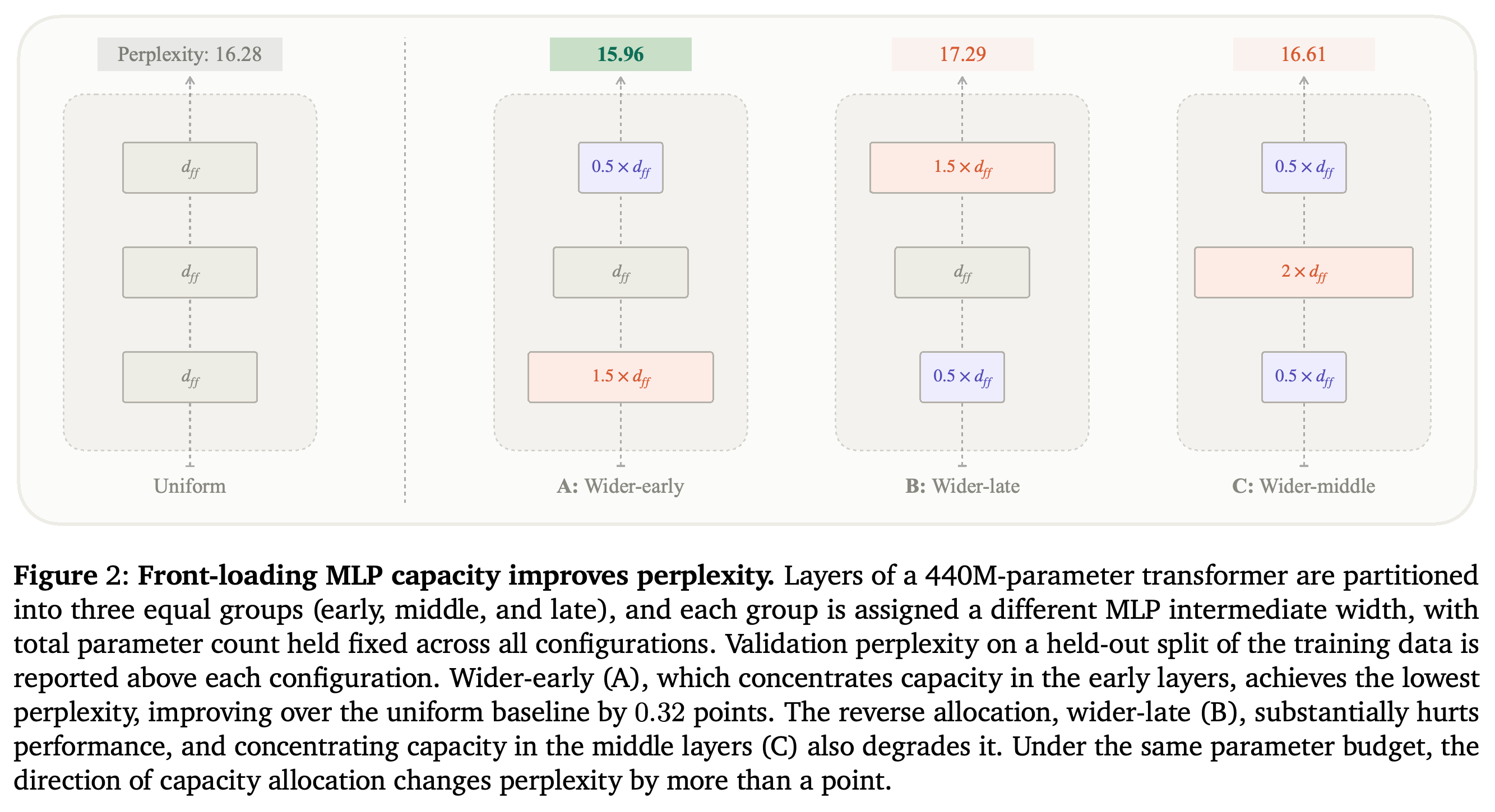
The motivating experiment divides a 440M Transformer into three equal groups of early, middle, and late layers. At a fixed total parameter count, the uniform allocation reaches 16.28 perplexity, wider-early reaches 15.96, wider-late reaches 17.29, and wider-middle reaches 16.61.

In early-to-late order, wider-early assigns width multipliers 1.5, 1, and 0.5; wider-late assigns 0.5, 1, and 1.5; wider-middle assigns 0.5, 2, and 0.5.
The opposite outcomes of wider-early and wider-late support a directional allocation effect rather than a benefit from non-uniformity alone. This experiment establishes that effect for the tested Transformer, not for every model family.

Uniform, wider-early, wider-late, and wider-middle MLP allocations across three equal layer groups of a 440M Transformer.

2. Tapered Language Models

Tapered Language Models (TLMs) extend the three-group intervention into a fixed architectural allocation that decreases a parameter-bearing dimension monotonically across layers. The experiments instantiate this principle exclusively through MLP intermediate width, whose parameter count varies linearly with width across the considered architectures.

Attention head count, key-value dimension, recurrent state size, memory slot count, and Mixture-of-Experts expert count are proposed as other candidate dimensions, but are not experimentally tapered in this paper.

2.1. Background

For a decoder-only model with L blocks and residual dimension d, the paper writes each block as (z_l = h_l + \mathcal{M}l(h_l)), followed by (h{l+1} = z_l + \mathcal{F}_l(z_l)), omitting layer normalization for brevity. The token mixer M varies by architecture, whereas the MLP F exposes an intermediate dimension d_ff that controls its capacity.

The per-layer MLP parameter count is 2 d d_ff for vanilla FFNs and 3 d d_ff for SwiGLU. Both are linear in d_ff, enabling budget-preserving redistribution without changing the residual dimension.
Typical uniform widths are 4d for standard FFNs and (8/3)d for gated variants.

2.2. Tapering

For layer indices l ∈ {0, 1, …, L − 1}, tapering requires d_C(l + 1) ≤ d_C(l) for adjacent layers and (1/L) ∑_{l=0}^{L−1} d_C(l) = d_C^baseline. The first condition fixes the early-to-late allocation direction; the second preserves the component’s average dimension.

For the tested MLP intervention, preserving average width preserves parameter count because the projections scale linearly with that width. The general formulation does not demonstrate that every proposed component has the same relationship between dimension and cost.

2.3. Tapering MLP Width

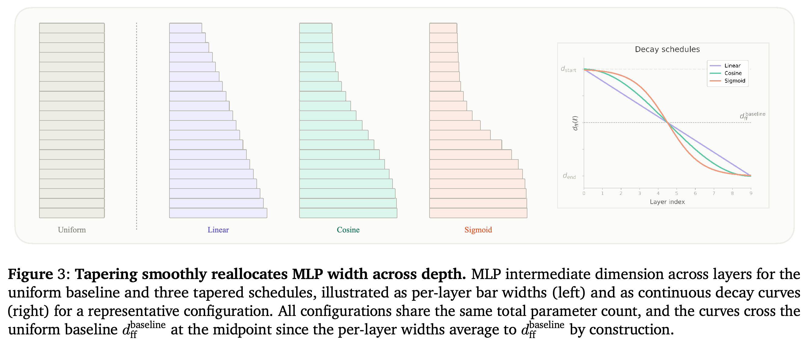
The paper compares linear, cosine, and sigmoid schedules parameterized by d_start > d_end. Linear spreads the reduction at a constant rate; cosine changes slowly near the endpoints and most rapidly around the midpoint; sigmoid concentrates the transition around the middle, with k = 10 in every experiment.

Linear: d_ff(l) = d_start − (d_start − d_end) l/(L − 1).
Cosine: d_ff(l) = d_end + ((d_start − d_end)/2)(1 + cos(πl/(L − 1))).
Sigmoid: d_ff(l) = d_end + (d_start − d_end)/(1 + exp(k(l/(L − 1) − 0.5))).

Parameter preservation requires (1/L) ∑_{l=0}^{L−1} d_ff(l) = d_ff^baseline. Since MLP parameter counts and projection FLOPs are linear in intermediate width, this constraint redistributes rather than increases the total parameter and FLOP budgets.

Widths are rounded to the nearest multiple of 16. The first and last widths are fixed to d_start and d_end, and interior widths are adjusted in 16-unit increments to satisfy the budget exactly while retaining monotonic order.
Residual dimension, attention head count, and key-value dimension remain identical to the baseline. Equal FLOPs do not establish equal wall-clock latency or throughput.

Per-layer MLP width profiles and continuous linear, cosine, and sigmoid decay curves relative to a uniform baseline.

3. Experiments

The experiments separate configuration selection from transfer evaluation. A 440M Transformer is used for the schedule and width sweep, after which the selected configuration is evaluated unchanged across four architectures at 760M and 1.3B.

Within each uniform–tapered comparison, total parameters, training FLOPs, inference FLOPs, and training hyperparameters are held fixed; only the per-layer MLP intermediate dimension changes.

3.1. Setup

The four backbones are Transformer with standard softmax self-attention, Gated Attention with output gating, Hope-attention with self-modifying memory operating at multiple frequencies, and Titans with a neural long-term memory module that learns to memorize at test time. This selection tests whether the same MLP allocation transfers across different token mixers.

Training uses the Llama 3 tokenizer with a reported vocabulary size of 32K and sequences of 4K tokens. The 440M, 760M, and 1.3B models receive 30B, 50B, and 100B training tokens, respectively.

The optimizer is AdamW with cosine annealing, a peak learning rate of 4 × 10−4, weight decay of 0.1, and a global batch size of 0.5M tokens.
The PDF states that training uses accelerator hardware, but does not specify the accelerator model or identify the pretraining corpus.

Schedule selection uses in-distribution perplexity on a held-out split of the training data. Main evaluation uses out-of-distribution perplexity on WikiText and LAMBADA, together with accuracy on LAMBADA, PIQA, HellaSwag, WinoGrande, ARC-easy, ARC-challenge, SIQA, and BoolQ.

Table 2 labels HellaSwag and ARC-challenge with acc_n, distinguishing these columns from the other accuracy columns. Avg. is the mean across the eight reported task scores.

3.2. Schedule and Width Sweep

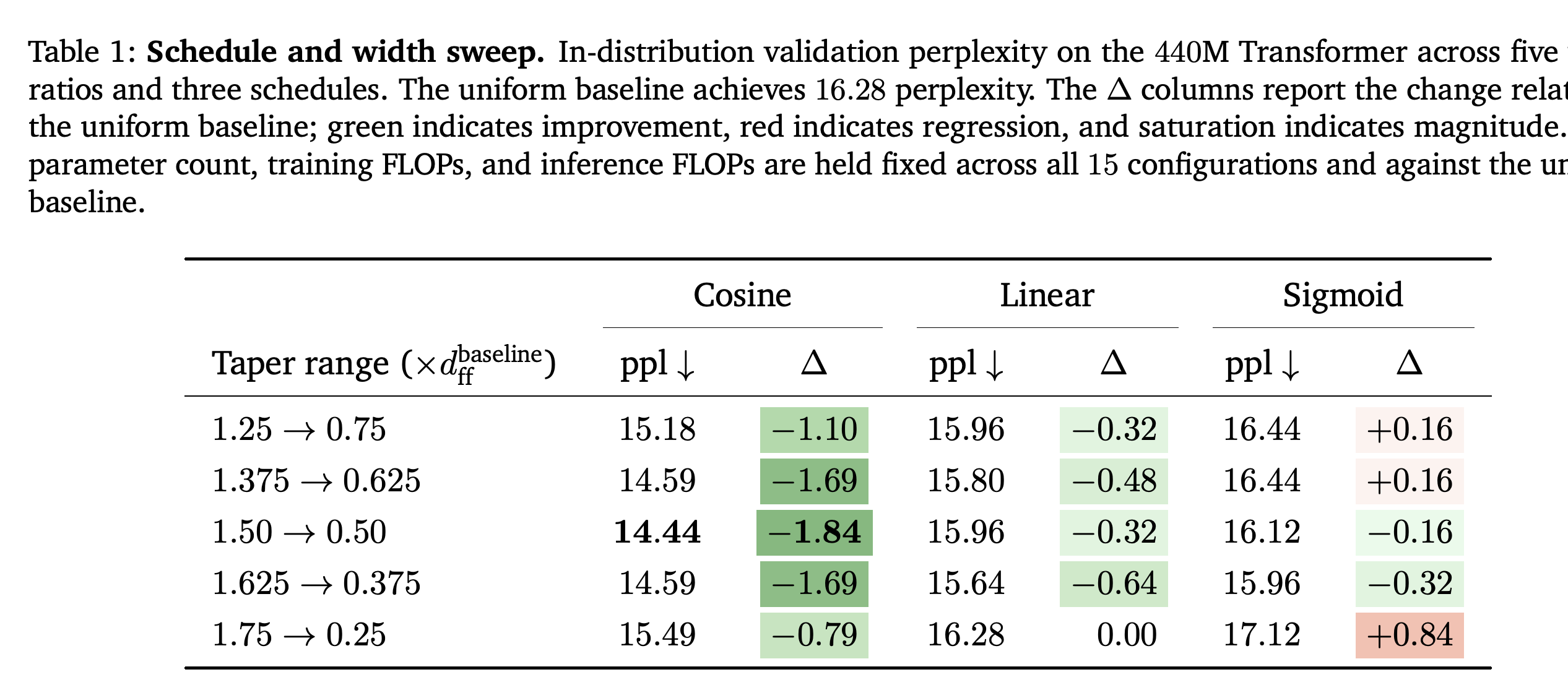
The 440M Transformer sweep combines three schedules with five start-to-end ranges: 1.25→0.75, 1.375→0.625, 1.50→0.50, 1.625→0.375, and 1.75→0.25 times the baseline width. Cosine has the lowest perplexity at every range; linear outperforms sigmoid at four ranges and ties it at 1.625→0.375, where both reach 15.96.

Cosine perplexities in range order are 15.18, 14.59, 14.44, 14.59, and 15.49. The minimum improves on the 16.28 uniform baseline by 1.84 points, while more aggressive redistribution loses some of that benefit.
Even the worst tested cosine result, 15.49, is better than the best tested linear result, 15.64. Sigmoid can regress relative to uniform allocation, reaching 17.12 at 1.75→0.25.
The selected cosine range, 1.50→0.50, is a default selected at one operating point, not an established global optimum. The authors’ explanation in terms of endpoint plateaus and a gradual middle transition is not independently isolated by the sweep.

In-distribution validation perplexity and changes from the 16.28 uniform baseline for three schedules and five taper ranges on a 440M Transformer.

3.3. Language Modeling and Commonsense Reasoning

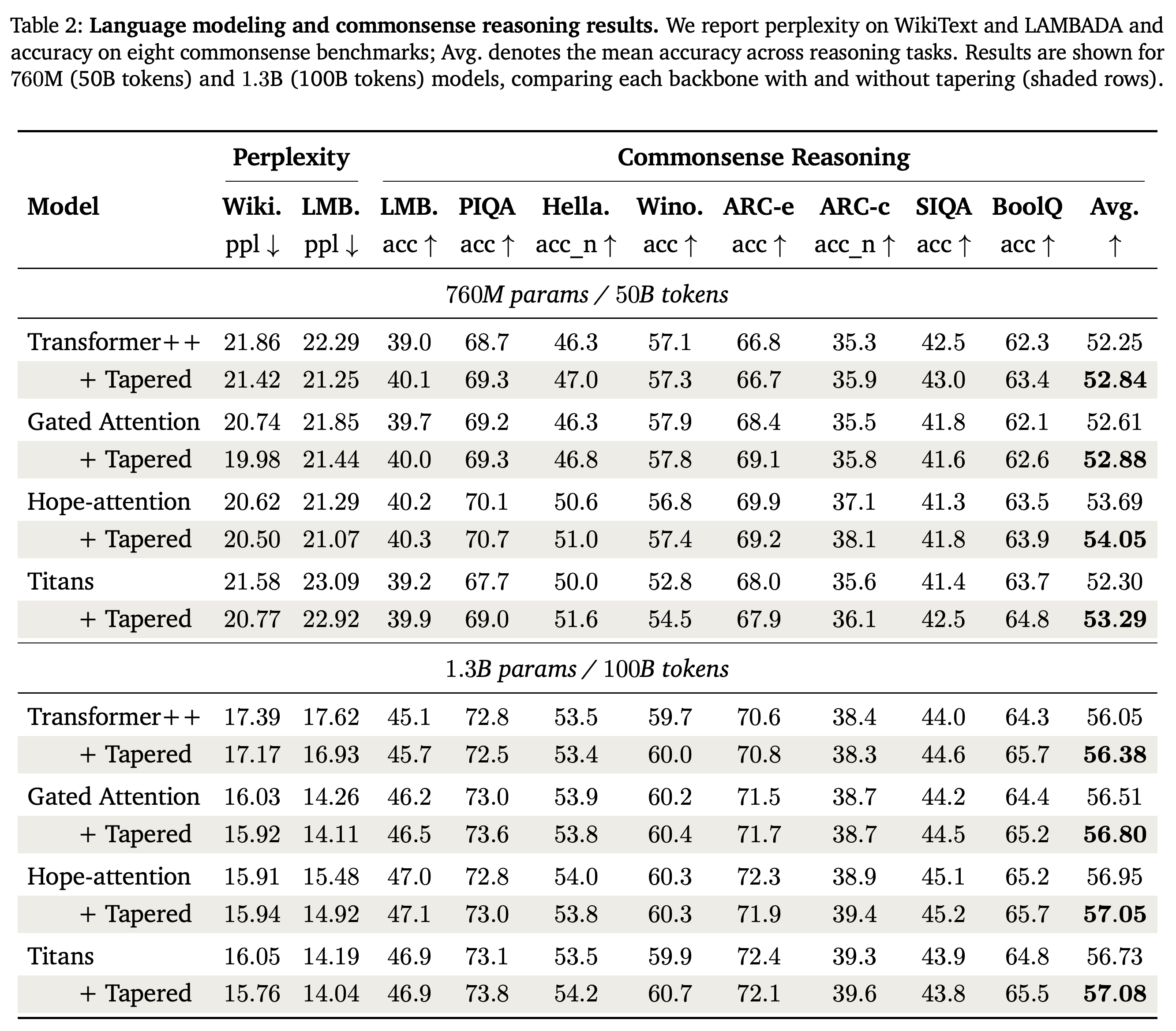
With the selected cosine taper held fixed, Table 2 reports higher average commonsense accuracy for every backbone at both larger scales. LAMBADA perplexity decreases in all eight comparisons; WikiText perplexity decreases in seven, with 1.3B Hope-attention increasing slightly from 15.91 to 15.94.

At 760M, Avg. changes from 52.25 to 52.84 for Transformer++, 52.61 to 52.88 for Gated Attention, 53.69 to 54.05 for Hope-attention, and 52.30 to 53.29 for Titans.
At 1.3B, Avg. changes from 56.05 to 56.38 for Transformer++, 56.51 to 56.80 for Gated Attention, 56.95 to 57.05 for Hope-attention, and 56.73 to 57.08 for Titans.
Individual task scores do not improve uniformly. For example, 1.3B Transformer++ PIQA decreases from 72.8 to 72.5, and 1.3B Hope-attention ARC-easy decreases from 72.3 to 71.9; the consistent result concerns task averages rather than every benchmark.

WikiText and LAMBADA perplexity and eight task scores for uniform and tapered backbones at 760M parameters with 50B training tokens and 1.3B parameters with 100B training tokens.

4. Layer-wise Novelty

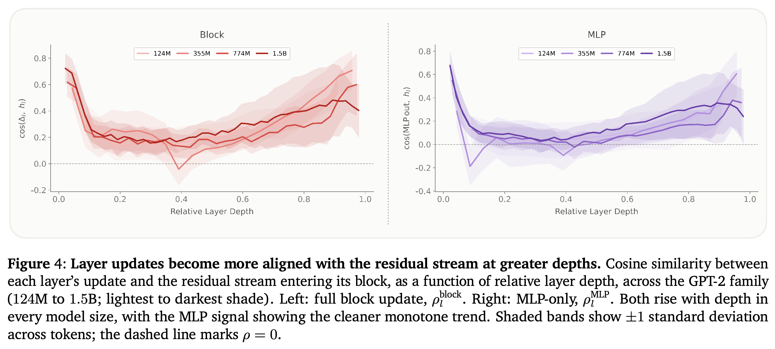
Layer-wise novelty is assessed using two token-averaged cosine similarities: ρ_l^block = cos(h_{l+1} − h_l, h_l) and ρ_l^MLP = cos(F_l(z_l), h_l). The first measures alignment of the full block update with the incoming residual; the second isolates the MLP contribution.

A value near zero indicates an update orthogonal to the reference residual, while a positive value indicates alignment with a direction already present. The paper interprets increasing alignment as decreasing novelty; this is a directional proxy rather than a direct measure of information content.
Both metrics use h_l as their reference, even though the MLP output is added to z_l. The stated reason is to share an unnormalized reference and avoid directional distortion from the normalized MLP input.

The analysis uses 2048 tokens from WikiText-2 and pretrained GPT-2 checkpoints spanning 124M to 1.5B parameters, excluding first and last layers as boundary cases. Both block and MLP alignment fall to low values in early-middle layers and generally increase through the second half of each model.

Pearson correlations with layer index are positive in every measurement: r = 0.49 to r = 0.71 for the MLP metric and r = 0.27 to r = 0.71 for the block metric.
These measurements support a depth-dependent change in update direction. They do not directly measure unused hidden dimensions or prove that aligned updates are unnecessary, and they analyze GPT-2 rather than the four experimentally tapered backbones.

Full-block and MLP-only cosine alignment with the incoming residual across relative layer depth in GPT-2 models from 124M to 1.5B, with ±1 standard deviation across tokens.

The paper distinguishes static MLP tapering from token-dependent compute routing, sequence pooling, layer dropping, elastic nested blocks, and post-training pruning. Its closest comparisons are earlier methods that redistribute FFN capacity across layers, sometimes jointly changing attention dimensions or removing FFNs altogether.

The methodological distinction is an isolated MLP-width intervention at equal parameter and FLOP budgets, with every layer remaining active. This avoids conflating width redistribution with changed effective depth or simultaneous changes to multiple architectural dimensions.
Prior work does not uniformly favor early allocation: the discussion notes a study whose headline result favors middle placement, with placement preferences varying by scale. Controlled conditions therefore matter when interpreting the direction of tapering.
Early-exit, redundancy, and FFN interpretability studies motivate non-uniform layer importance, but are not substitutes for the paper’s fixed-budget architectural experiments.

6. Limitations

The paper’s explicit limitation is that the schedule and endpoint search is performed only on the 440M Transformer. Transferring the selected configuration unchanged provides evidence of transferability, but does not establish optimality for the larger models or alternative architectures.

The preferred profile may depend on depth, hidden dimension, the MLP parameter fraction, token-mixing architecture, and training budget.
An additional evaluation limitation is that the PDF reports no repeated-seed variability or confidence intervals for the benchmark comparisons. The small average-score changes cannot therefore be assessed for statistical reliability from the reported results alone.
The mechanism study uses a short WikiText-2 sample and a separate pretrained model family; it does not test a causal link between measured alignment and the improvements from tapering.

7. Discussion and Conclusion

A fixed cosine allocation of MLP width improves aggregate evaluation results across the tested backbones and budgets without increasing total parameters or FLOPs. The coarse allocation experiment, schedule sweep, and transfer evaluations support reconsidering uniform MLP capacity across depth under these conditions.

Tapering other dimensions, and applying the principle to vision transformers, diffusion transformers, or multimodal models, remain proposed extensions rather than demonstrated results.
The experiments cover three parameter scales overall, but the full four-architecture language-modeling and reasoning comparison covers only 760M and 1.3B.

Appendix

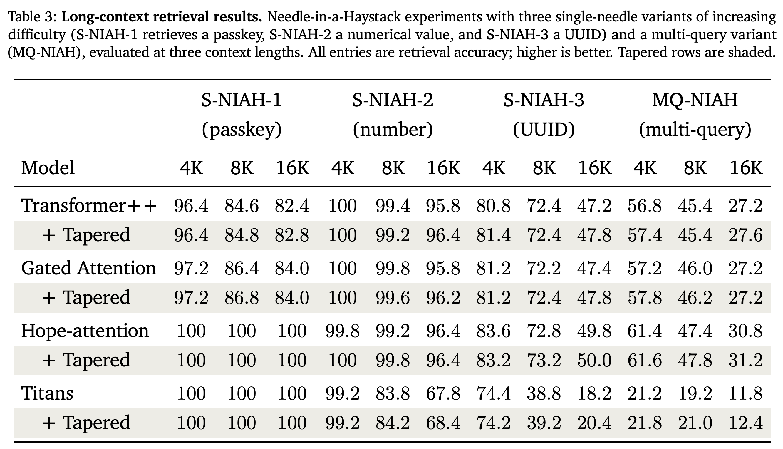
A. Long-Context Retrieval on Needle-in-a-Haystack evaluates S-NIAH-1 for passkeys, S-NIAH-2 for numerical values, S-NIAH-3 for UUIDs, and MQ-NIAH for multiple queries, each at 4K, 8K, and 16K context lengths. Table 3 generally shows unchanged or modestly improved retrieval accuracy; for example, Titans S-NIAH-3 at 16K rises from 18.2 to 20.4. However, the appendix’s statement that tapered models match or improve across the table overlooks several declines, including Transformer++ S-NIAH-2 at 8K from 99.4 to 99.2 and Hope-attention S-NIAH-3 at 4K from 83.6 to 83.2; the appendix does not identify the evaluated parameter scale.

Brief Thoughts

The main contribution is the controlled isolation of where MLP capacity is placed. The allocation-direction experiment and unchanged transfer across four backbones provide evidence that uniform width is not always the best choice at a fixed parameter and FLOP budget.

The evidence does not establish that later layers cannot use additional capacity: cosine alignment is a directional proxy, and the main-table gains include small improvements and individual regressions. Table 3 likewise supports broadly preserved retrieval behavior rather than improvement in every cell. Broader schedule searches, repeated-seed evaluations, and measured runtime comparisons would clarify optimality, reliability, and practical cost.

Needle-in-a-Haystack retrieval accuracy for passkey, numerical-value, UUID, and multi-query tasks at 4K, 8K, and 16K context lengths across four uniform and tapered backbones.