Communication-Efficient Language Model Training Scales Reliably and Robustly: Scaling Laws for DiLoCo | Summary

This article explains the key points of Communication-Efficient Language Model Training Scales Reliably and Robustly: Scaling Laws for DiLoCo.

• 2025-03-12 (arXiv)
• Charles, Zachary, Teston, Gabriel, Dery, Lucio, Rush, Keith, Fallen, Nova, Garrett, Zachary, Szlam, Arthur, Douillard, Arthur.
• Google Research, Google Search, Google DeepMind
• Paper

Read this article in Korean

Summary

• Frequent synchronization between devices can slow language model training, raising the question of whether less frequent synchronization preserves quality as models grow. DiLoCo, short for Distributed Low-Communication, periodically synchronizes independently trained model copies and achieves lower held-out loss, measured on data excluded from training, than Data-Parallel training, which synchronizes gradients every step, at 4B and 10B parameters with two model copies and the same model size and token budget.
• The authors fit scaling laws, empirical functions predicting loss and suitable training settings, using hyperparameter sweeps from 35M to 2.4B parameters and test predictions beyond that range at 4B and 10B. DiLoCo tolerates larger global batches, the tokens processed across all model copies per step, while its best outer learning rate, the step size for periodic synchronization updates, depends primarily on replica count and synchronization cadence, the number of local steps between updates, rather than model size.
• The loss improvements are small: with hyperparameters predicted jointly from model size and replica count, two-replica DiLoCo reaches 2.220 versus 2.224 at 4B and 2.086 versus 2.090 at 10B. Larger predicted speed advantages arise from reduced communication and increased parallelism, but the wall-clock comparisons use idealized models rather than measured deployments across datacenters.

1 Introduction

Communication-Efficient Language Model Training Scales Reliably and Robustly: Scaling Laws for DiLoCo studies how communication-efficient pretraining changes with model size. Previous DiLoCo results did not establish how its additional optimization settings should transfer to larger models, where exhaustive tuning becomes expensive.

• The study predicts held-out evaluation loss and optimal hyperparameters as functions of parameter count N and, for DiLoCo, replica count M.
• Most experiments fix synchronization cadence H = 30 and adopt the Chinchilla token allocation D = 20N, meaning 20 training tokens per model parameter.

2 Preliminaries

The notation separates model weights θ, parameter count N, evaluation loss L, training steps T, token budget D, and total floating-point operations C. DiLoCo additionally uses M model replicas, synchronization cadence H, inner learning rate γ for local updates, outer learning rate η, and global batch size B measured in tokens.

2.1 DiLoCo: Distributed Low-Communication

DiLoCo uses two levels of optimization: replicas independently update their local models for H inner steps, then synchronize through an outer optimizer. Each replica computes the difference between the previous global model and its current local weights; these differences are averaged, and the outer optimizer produces a new global model that replaces every replica’s local weights.

• The difference is Δ_m^(t) = θ^(t−H) − θ_m^(t), and its average is Δ^(t) = (1/M) Σ_m Δ_m^(t). Replicas retain their inner optimizer state across synchronization rounds.
• The authors call the averaged difference an outer gradient, while explicitly noting that it generally is not the gradient of any function.

Four independent training paths meet at outer updates. Synchronization combines accumulated model differences after several local steps, changing the optimization trajectory as well as communication frequency.

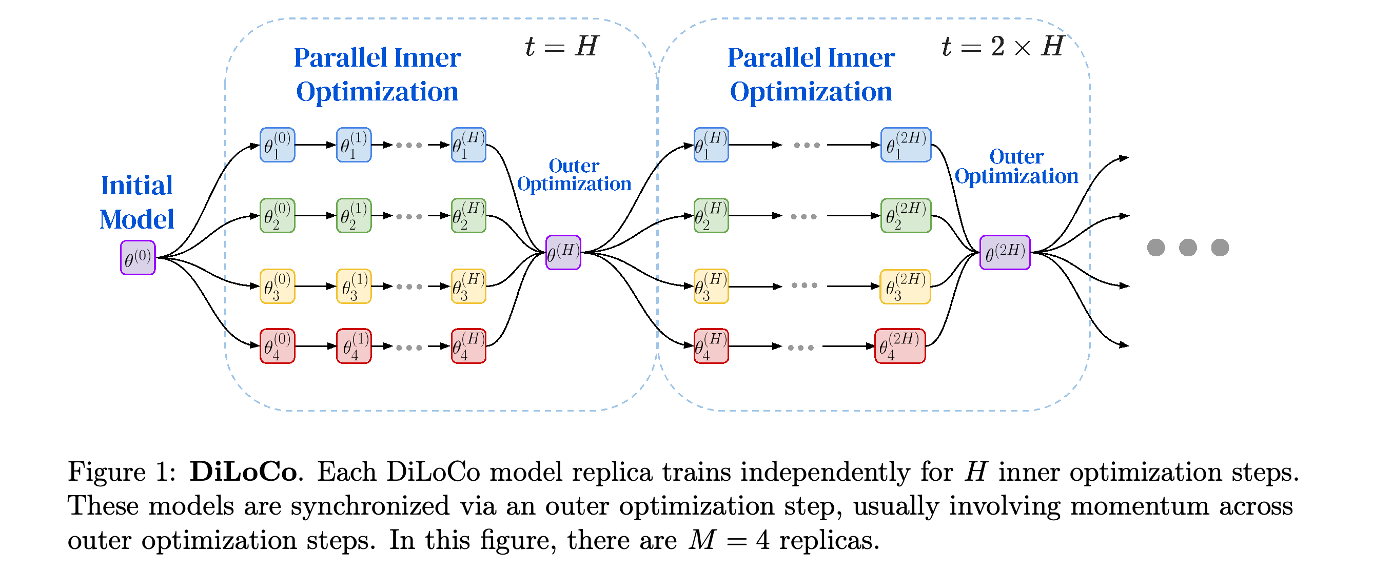
2.2 Data-Parallel versus DiLoCo

Data-Parallel computes one synchronized gradient update from B tokens per step. DiLoCo splits the same global batch across M replicas, giving each replica B/M tokens, and applies its outer update every H steps.

• Comparisons hold N and total D constant; evaluation uses the current Data-Parallel model and the most recent DiLoCo global model.
• With M = 1, DiLoCo still performs outer optimization. It becomes a variant of Lookahead, an optimizer that periodically updates a slow model from locally trained weights, with an additional infrequent momentum operation in the configuration studied here.

3 Experimental Methodology

The experiments train Chinchilla-style decoder-only transformers, language models that predict subsequent tokens, from scratch with a vocabulary of 32,768 and maximum sequence length 2,048. QK-LayerNorm, normalization of attention queries and keys, reduces learning-rate sensitivity, while the z-loss regularization term is used to improve training stability.

• Most training uses C4, a text pretraining dataset, with loss evaluated on its held-out validation split. Downstream zero-shot evaluation, testing without task examples supplied at evaluation, covers HellaSwag sentence completion, Piqa physical commonsense reasoning, and Arc-Easy question answering.
• Data-Parallel and DiLoCo’s inner optimizer use AdamW, adaptive optimization with decoupled weight decay, with β₁ = 0.9, β₂ = 0.99, 1000 warmup steps, cosine decay to 5% of peak learning rate, weight decay T^−1, and inner-gradient norm clipping at 1.
• The outer optimizer uses stochastic gradient descent with Nesterov momentum 0.9, which carries information across outer updates, constant η, and no outer-gradient clipping. A modified NanoDO language-model implementation uses DrJAX for replica parallelism, all-reduce operations that aggregate updates across devices, bfloat16 numerical representations for weights and gradients, and TPUv5e, TPUv6e, and TPUv5 accelerators.

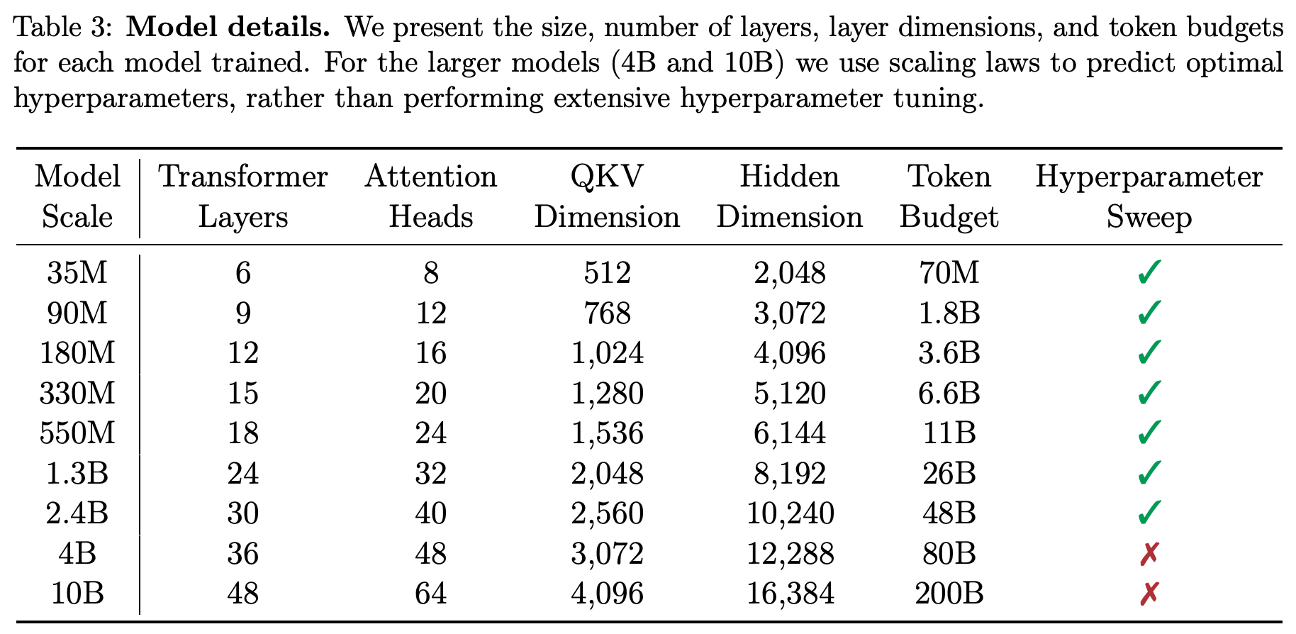
The table separates the models used for extensive tuning from the 4B and 10B extrapolation experiments. Its 35M token-budget entry and 330M model label differ from the default allocation and later labeling, so those entries require qualification.

3.1 Scaling Law Experiments

Hyperparameter sweeps cover models from 35M to 2.4B parameters, using integer powers of √2 for γ and powers of 2 for B. DiLoCo additionally sweeps M ∈ {1,2,4,8} and η ∈ {0.2,0.4,0.6,0.8,1.0}; grids expand until the lowest loss lies at an interior point.

• The 4B and 10B models use predicted hyperparameters rather than extensive sweeps, with token budgets of 80B and 200B respectively.
• The declared default D = 20N means doubling B halves the number of training steps at fixed N. Table 3 nevertheless lists 70M tokens for the 35M model and labels the intermediate model 330M where later results use 335M; these are inconsistencies in the source.

4 Empirical Findings

Finding 1: Scale. DiLoCo’s loss relative to Data-Parallel generally improves with model size, although multiple replicas often incur a small loss penalty at smaller scales. At 2.4B, two-replica DiLoCo reaches 2.323 versus 2.326 for Data-Parallel; four and eight replicas remain worse at 2.332 and 2.351.

• Table 5 reports lower losses at 4B and 10B for M = 1 and M = 2 using scaling-law hyperparameters, while M = 4 remains slightly worse.
• The quality advantage depends on model size, replica count, and the selected hyperparameters.

Absolute losses are close, but the relative-loss panel shows that the penalty from multiple replicas shrinks with scale. The two-replica curve crosses below the Data-Parallel baseline at the largest tuned size.

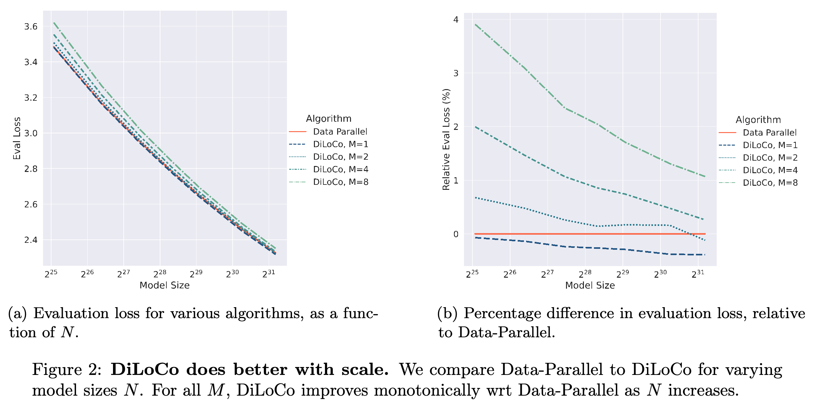
The results distinguish the consistent small advantage of M = 1 from the scale-dependent trade-off at larger M. At 2.4B, M = 2 improves loss to 2.323 from 2.326, while M = 4 and M = 8 still incur penalties.

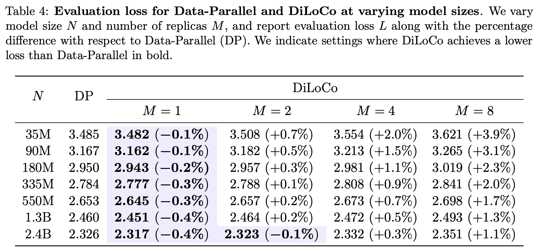
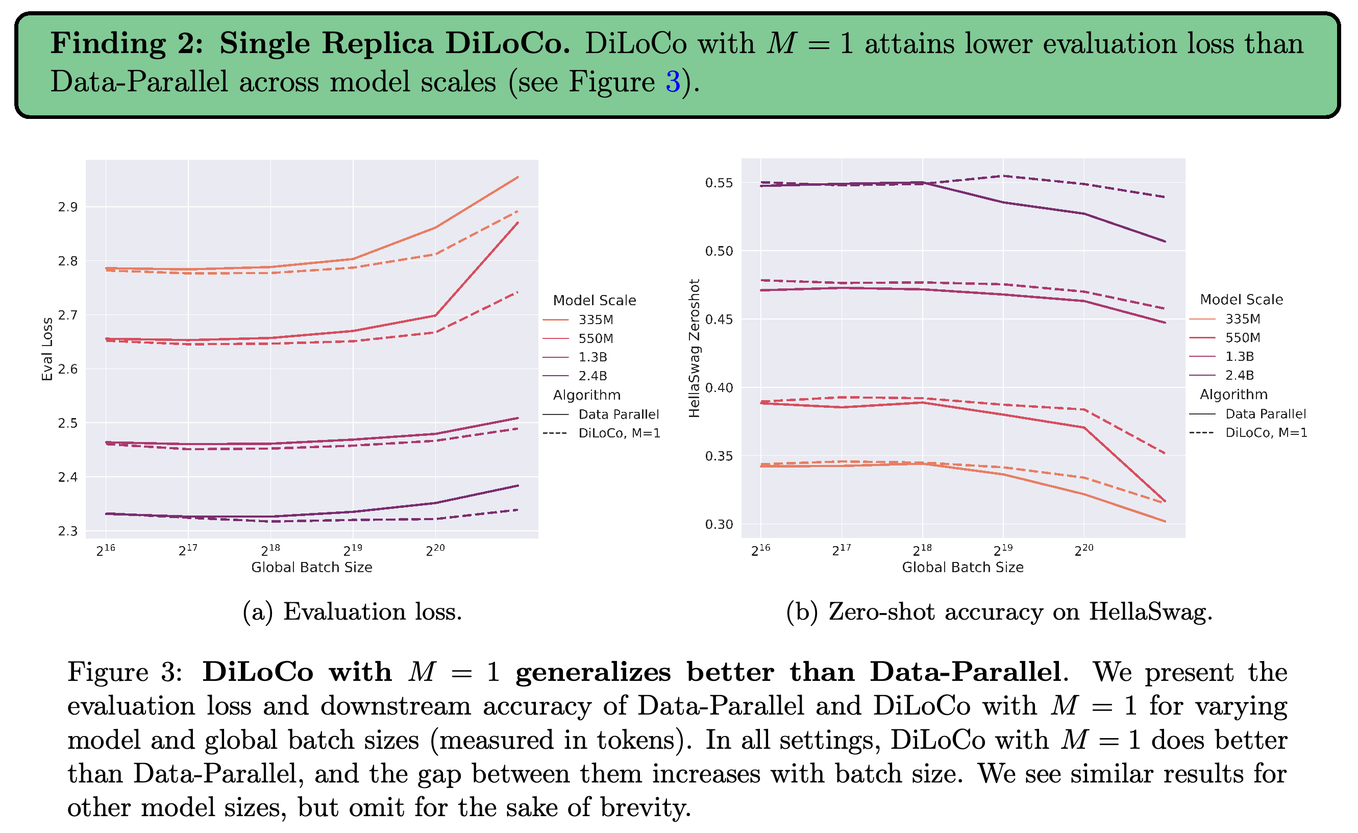
Finding 2: Single Replica DiLoCo. In the extensively tuned regime, M = 1 achieves lower best loss at every reported model size, from 3.482 versus 3.485 at 35M to 2.317 versus 2.326 at 2.4B. Its loss and HellaSwag accuracy also deteriorate less as batch size increases, showing an optimization benefit without communication reduction.

The single-replica comparison shows improved large-batch behavior without communication reduction. The separation becomes especially visible where Data-Parallel loss rises and HellaSwag accuracy falls at large batches.

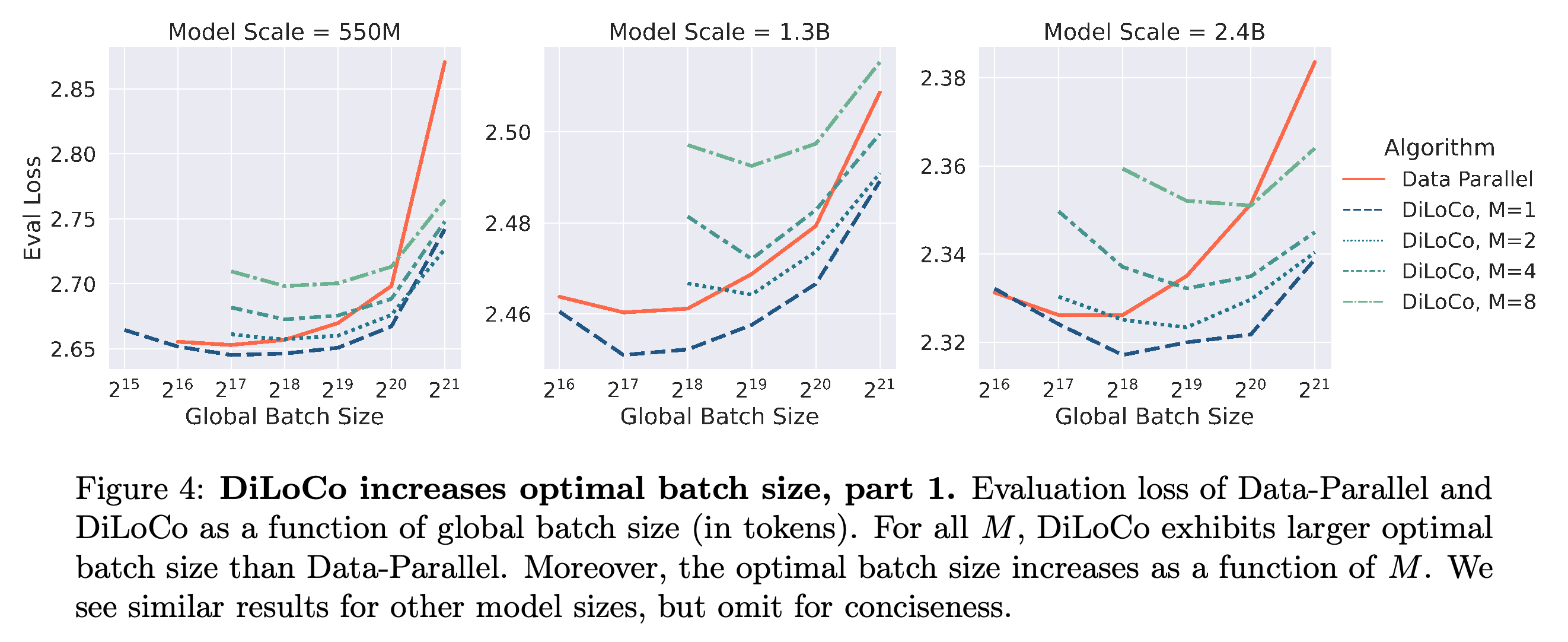
Finding 3: Optimal batch size. DiLoCo shifts the best global batch size upward, with larger replica counts generally supporting larger batches. Under a fixed token budget, this permits fewer sequential training steps and greater horizontal scalability, meaning more computation can run concurrently.

• Figures 4 and 5 show that Data-Parallel quality declines faster at large batches; DiLoCo with M > 1 can therefore outperform it at large batches even when its best achievable loss across all batches is worse.
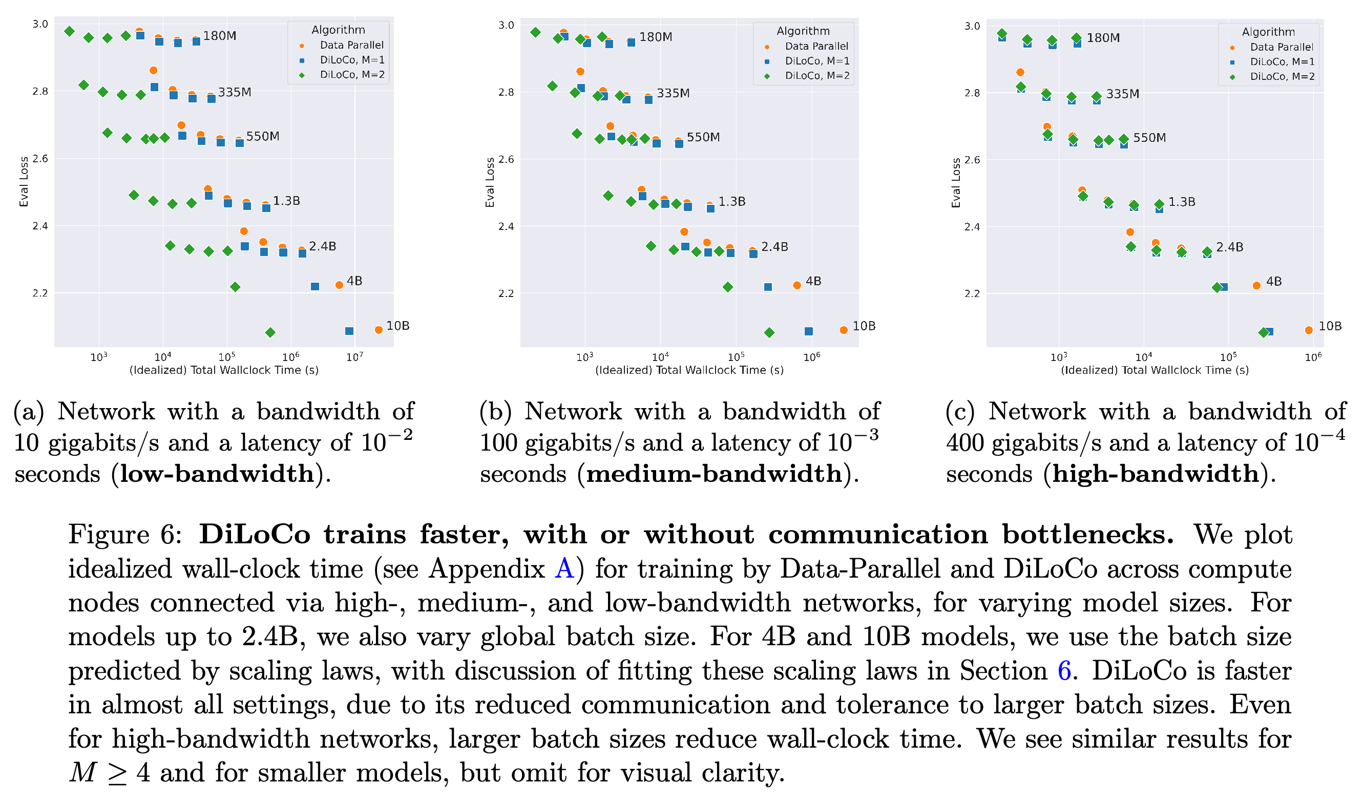
• Figure 6 predicts shorter wall-clock training under networks of 10 gigabits/s with 10^−2 seconds latency, 100 gigabits/s with 10^−3 seconds latency, and 400 gigabits/s with 10^−4 seconds latency. These predictions assume additional chips become available as batch size increases.

The minima generally shift toward larger global batches as replicas are added. Higher-replica curves can have worse minimum loss yet become preferable at large operating batches, distinguishing best quality from tolerance to additional parallelism.

DiLoCo points often lie to the left of comparable-loss Data-Parallel points, particularly under constrained bandwidth. These positions combine measured evaluation losses with modeled elapsed times, so the predicted speed gains depend on the stated network and resource assumptions.

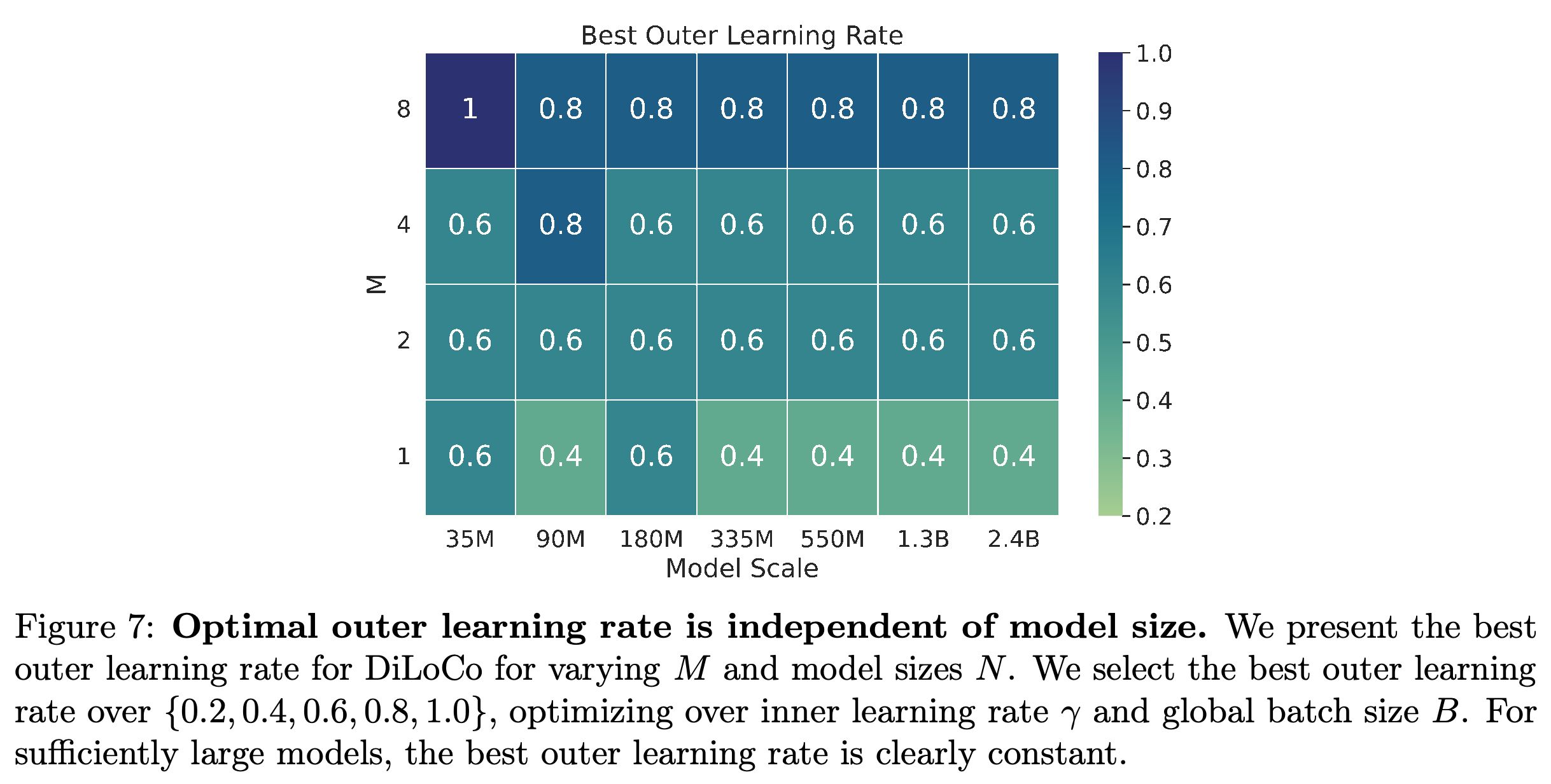
Finding 4: Outer learning rate. For N ≥ 335M and H = 30, the best tested η remains constant across model sizes: 0.4 for M = 1, 0.6 for M = 2 and M = 4, and 0.8 for M = 8. This supports selecting η at smaller scales while separately scaling the inner learning rate and batch size.

From 335M onward, each replica-count row has the same selected outer learning rate across model sizes. The heatmap supports transferring this setting across N within the tested grid while retaining its dependence on M.

5 Ablations

The ablations test whether the main findings persist when changing synchronization frequency and training on more tokens than the default allocation. They examine optimization behavior alongside simulated communication requirements.

5.1 Synchronization Cadence

The synchronization study sweeps H ∈ {1,5,10,30,100,300} and η ∈ {0.05,0.1,0.2,0.4,0.6,0.8,1.0}, retaining the previously selected inner learning rate and global batch size. The best outer learning rate increases with H and M while remaining approximately independent of N.

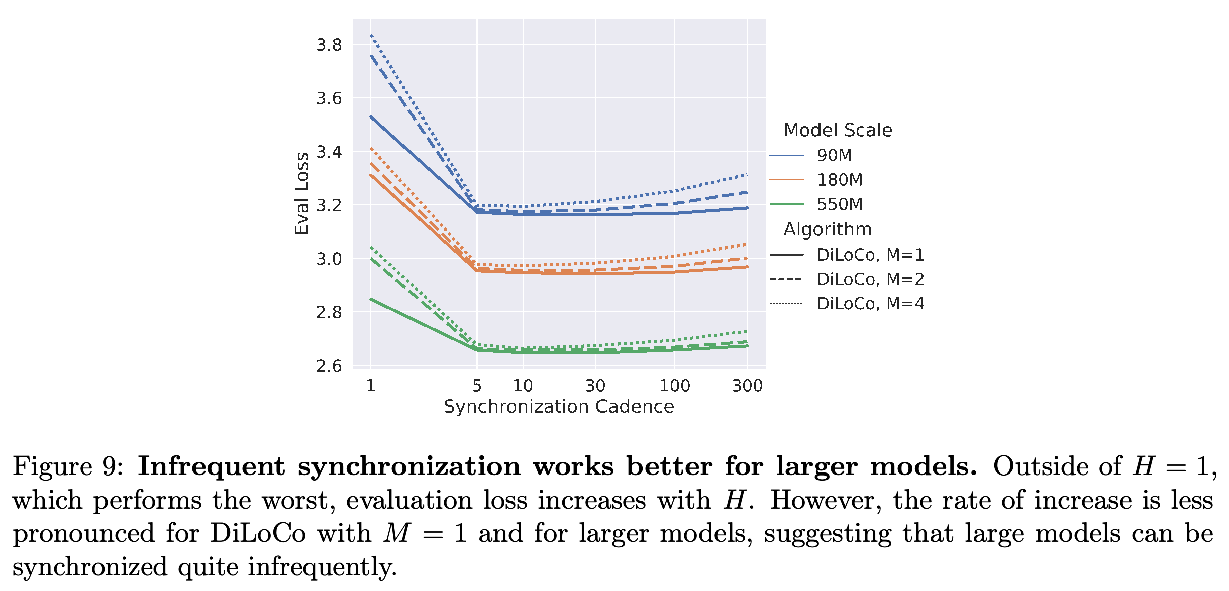
• H = 1 performs worst under this protocol. Beyond that setting, loss tends to increase with H, but the increase is smaller for larger models and M = 1.
• Because inner learning rate and batch size are not retuned for each H, the curves measure transfer of the selected settings rather than fully optimized performance at every cadence.

Loss is especially poor when synchronizing every step under the transferred inner settings. Longer intervals beyond the short-interval region produce smaller penalties for larger models, although the experiment does not retune all hyperparameters at each cadence.

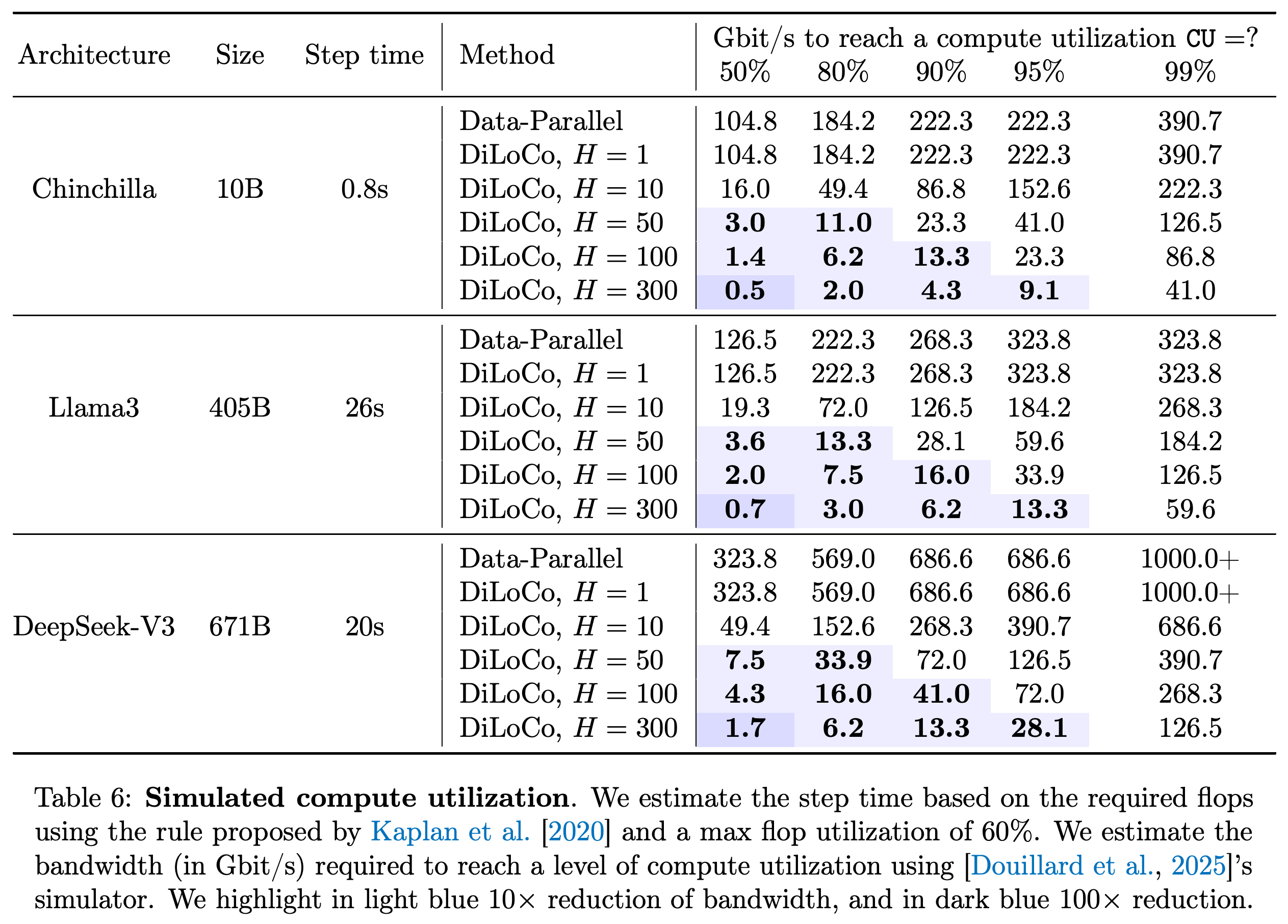
Compute utilization, defined here as computation time divided by total time, is simulated for 10B Chinchilla, 405B Llama3, and 671B DeepSeek-V3. Increasing H sharply reduces the inter-datacenter bandwidth needed for a given utilization.

• For 10B Chinchilla at 80% utilization, Table 6 gives 184.2 Gbit/s for Data-Parallel versus 2.0 Gbit/s for DiLoCo with H = 300. The corresponding values are 222.3 versus 3.0 Gbit/s for 405B Llama3 and 569.0 versus 6.2 Gbit/s for 671B DeepSeek-V3.
• These are simulator outputs using estimated step times and maximum floating-point-operation utilization of 60%; the study does not train the 405B and 671B models to establish their optimization quality.

Required bandwidth falls substantially as synchronization becomes less frequent. For 10B Chinchilla at 80% utilization, the comparison is 184.2 Gbit/s for Data-Parallel against 2.0 Gbit/s at H = 300; the larger architectures are simulated cases rather than additional training experiments.

5.2 Overtraining

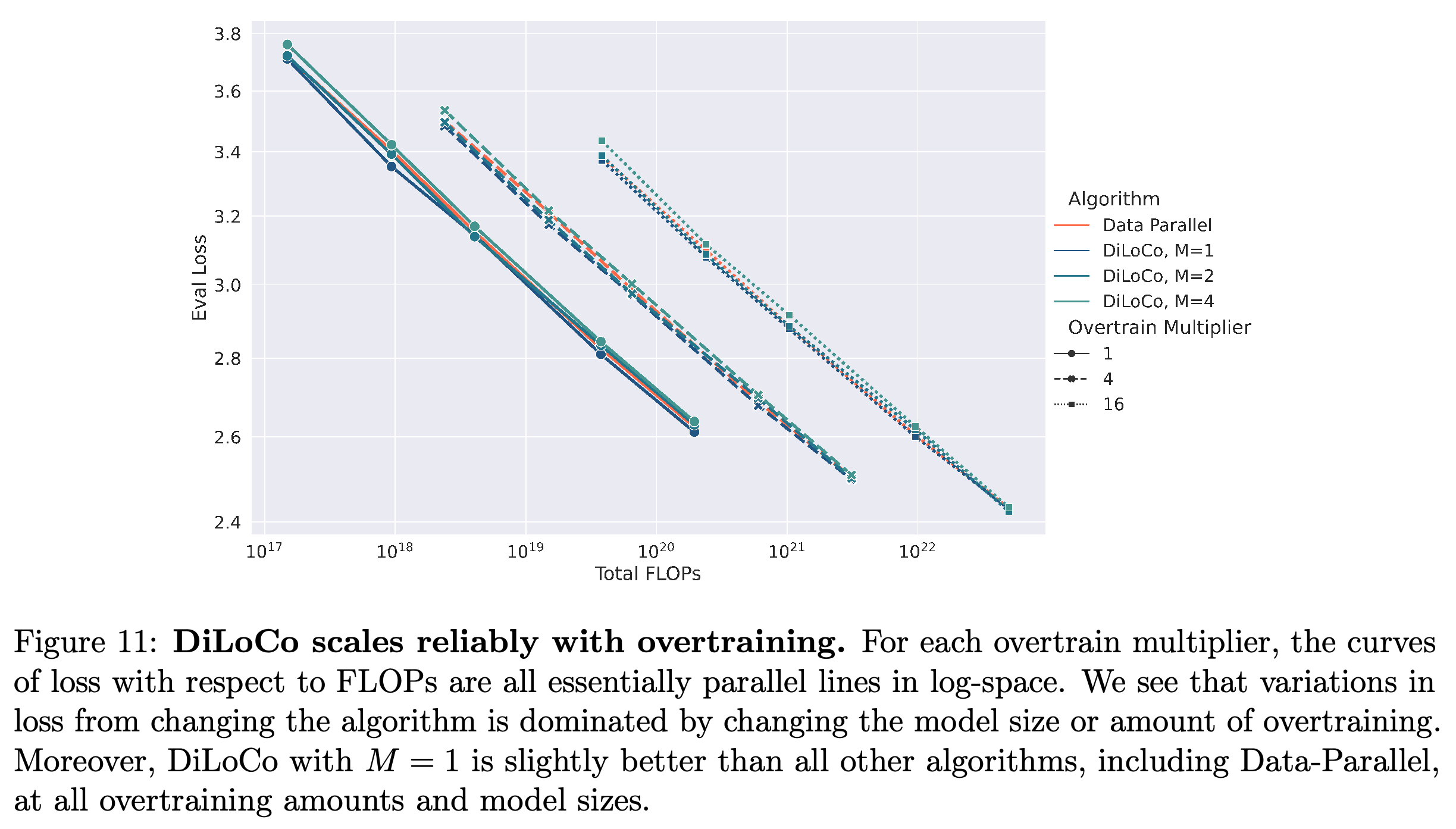
Overtraining means using more tokens than the Chinchilla allocation: D = 20Nλ with λ ∈ {1,4,16}. The authors train on Dolma, a larger text corpus, evaluate on C4 validation, and reuse the hyperparameters selected on C4 for Data-Parallel and DiLoCo with M ∈ {1,2,4}.

• Loss-versus-compute trends remain qualitatively similar across multipliers, and M = 1 remains slightly better in the displayed comparisons. Changes in model size and training-token allocation have larger effects than changing the algorithm.
• The idealized timing analysis for models from 335M to 2.4B predicts that M = 2 reduces elapsed time at all three network settings through larger batches and less frequent communication.

Changing the overtraining multiplier preserves similar loss-versus-compute trends across algorithms. This supports robustness of the scaling pattern when previously selected hyperparameters are reused on Dolma, without establishing that those settings remain optimal.

6 Scaling Laws

Scaling laws are fit to the minimum observed loss and associated hyperparameters for each model size and algorithm. The paper compares independent fits, which model each replica count separately, with joint fits, which model parameter count and replica count together.

6.1 Independent scaling laws

Independent loss fits use the power law L(N) ≈ AN^α, where A sets the scale and α determines how loss changes with model size. The fitted exponents are −0.0953 for Data-Parallel and −0.0961, −0.0969, −0.0992, and −0.1018 for DiLoCo with M = 1,2,4,8 respectively, indicating slightly steeper loss reductions for DiLoCo over the fitted range.

• Inner learning rates also receive power-law fits. To estimate optimal batch sizes between discrete sweep values, the authors first fit loss quadratically against log₂(B), then fit a power law to the resulting minima.
• Batch-size exponents are 0.281 for Data-Parallel and 0.435, 0.479, 0.510, and 0.455 for DiLoCo with M = 1,2,4,8. Outer learning rate is selected directly by M instead of fitting a dependence on N.

6.2 Joint scaling laws

Joint fits use f(N,M) ≈ AN^αM^β and linear regression in logarithmic coordinates. Table 10 reports L ≈ 19.226N^−0.0985M^0.0116, γ ≈ 22256N^−0.8827M^0.2929, and B ≈ 0.00709N^0.4695M^0.3399.

• Within this fitted form, replica count has a weak positive association with loss and a stronger positive association with optimal global batch size.
• These functions describe the tested token allocation and optimization protocol; their accuracy for arbitrary token budgets or untested replica counts is not established.

6.3 Measuring goodness-of-fit

Goodness-of-fit is tested by fitting through 1.3B parameters and predicting the held-out 2.4B setting. Prediction error is measured as res(y,ỹ) = |log(y) − log(ỹ)| for loss, inner learning rate, and global batch size.

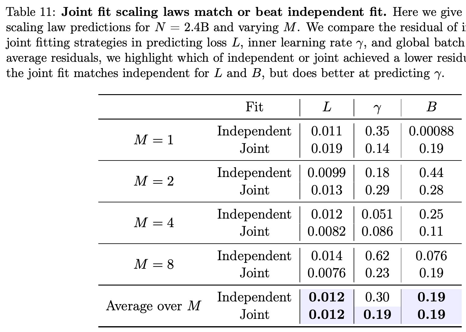
• Table 11 reports average residuals of 0.012 for loss and 0.19 for batch size for both approaches. For inner learning rate, the joint fit improves the average residual from 0.30 to 0.19.
• The paragraph in Section 6.3 reverses the learning-rate comparison in its prose; the numerical table and its caption support the joint fit.

The average errors distinguish prediction targets: loss and batch-size residuals match at displayed precision, while the joint fit reduces the inner-learning-rate residual from 0.30 to 0.19. These entries resolve the conflicting statement in the surrounding prose.

6.4 Extrapolating to larger models

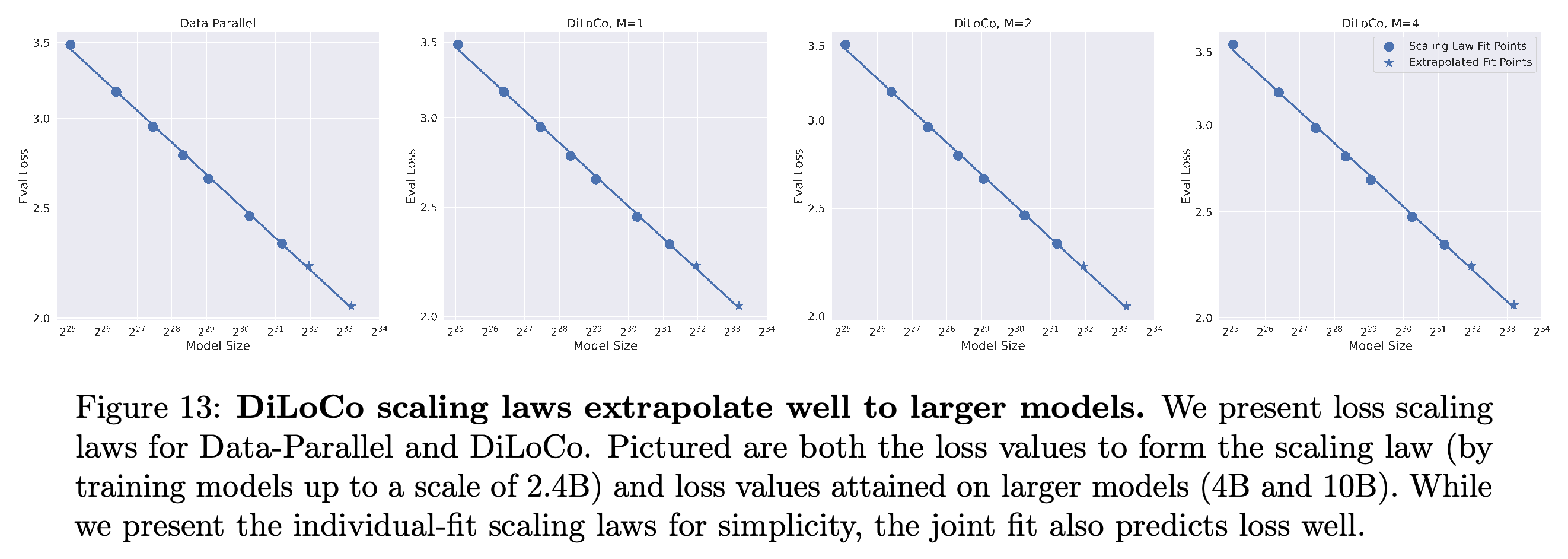
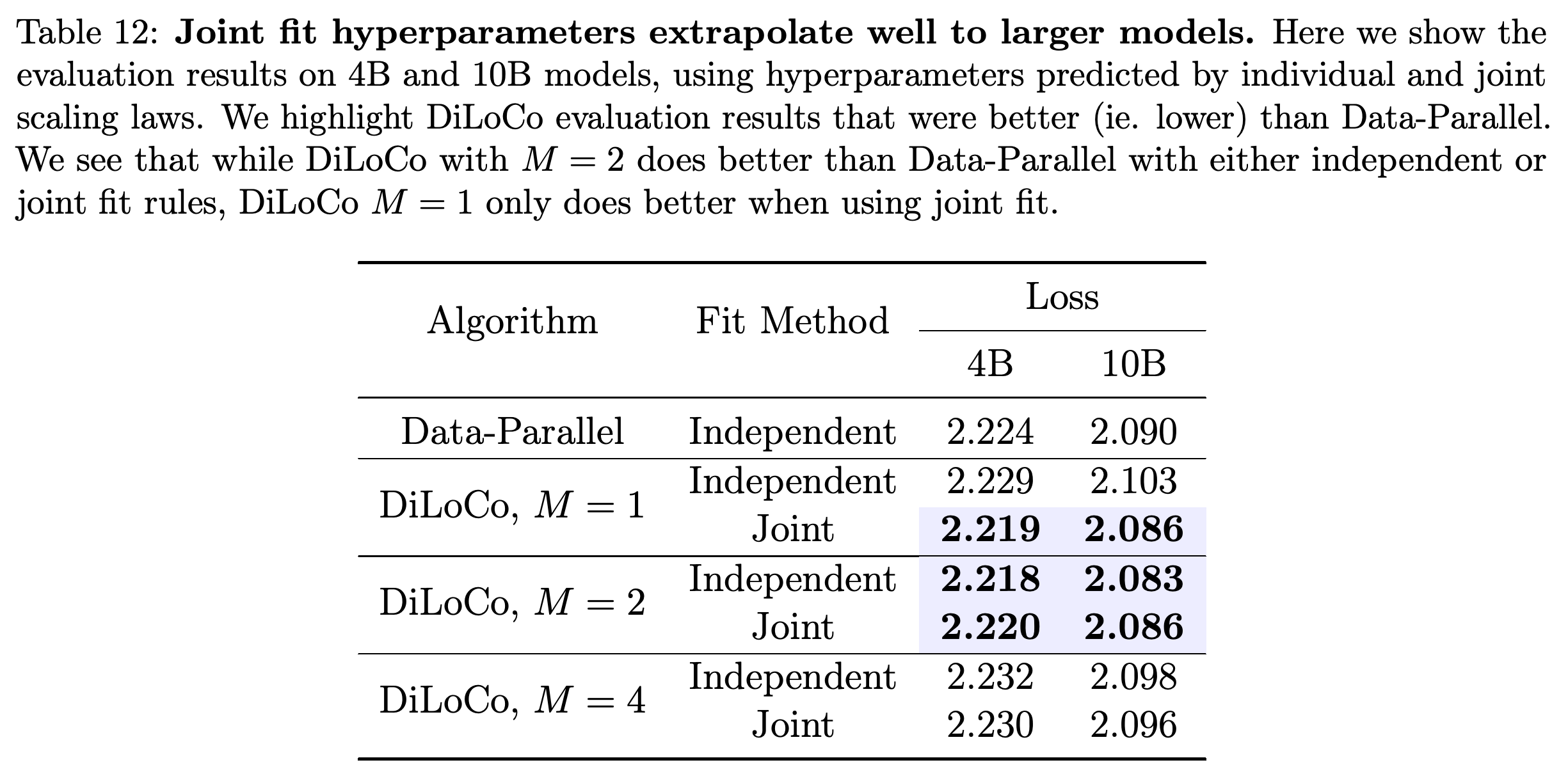
At 4B and 10B parameters, M = 2 beats Data-Parallel with either independent or joint hyperparameter fits. Independent fits yield losses of 2.218 and 2.083, while joint fits yield 2.220 and 2.086, compared with Data-Parallel’s 2.224 and 2.090.

• M = 1 only improves on Data-Parallel with joint-fit settings: 2.219 and 2.086 versus 2.229 and 2.103 with independent-fit settings. M = 4 remains slightly worse with either fit.
• Figure 13 shows that extrapolated losses remain near the fitted curves. The authors recommend joint hyperparameter fits overall, although Table 12 shows that independent fits give the best reported M = 2 losses at these two scales.

The 4B and 10B extrapolation markers remain near curves fitted using smaller models. This supports loss predictability over the evaluated extension, while numerical tables establish the smaller differences between algorithms.

Two replicas improve loss with either fitting strategy, whereas one replica improves only with joint-fit hyperparameters. Independent-fit M = 2 gives the lowest displayed losses, 2.218 and 2.083, so joint fitting does not always yield the best trained model.

6.5 Parametric Function Fitting

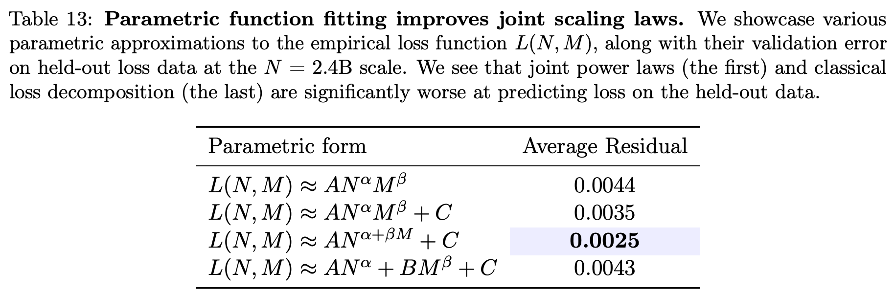
The authors compare four parametric loss functions: AN^αM^β, AN^αM^β + C, AN^(α+βM) + C, and AN^α + BM^β + C, where the letters denote fitted coefficients in these expressions. Parameters minimize Huber loss, an objective that reduces the influence of large residuals, on logarithmic prediction errors using L-BFGS, a numerical optimization method, from 256 random initializations.

• Held-out 2.4B data select the fitted parameters. Average residuals are 0.0044, 0.0035, 0.0025, and 0.0043 respectively, favoring AN^(α+βM) + C among the tested forms.
• The lowest-error form lets replica count change the exponent of model size. Because the held-out scale also guides selection, these residuals provide validation evidence rather than an independent final test of the selected function.

Allowing replica count to modify the exponent of model size gives the lowest validation residual, 0.0025, among the four candidate forms. The same held-out scale is used to select fitted parameters and compare their validation errors.

7 Related Work

The paper places DiLoCo among methods that reduce communication through infrequent updates, alongside Local SGD, stochastic gradient descent with periodic synchronization, and federated optimization. Federated learning trains over decentralized data, and its periodic averaging and inner/outer optimization schemes provide close algorithmic precedents.

• Other communication-reduction families use sparse updates, communicating a reduced update representation, or asynchronous updates, where workers need not synchronize at the same time. The present scaling laws concern the synchronous DiLoCo configuration studied experimentally.
• Relative to He et al. [2024], the authors study 10× larger models, multiple replica counts including M = 1, explicit token allocations and overtraining, hyperparameter scaling, and optimal batch size.

8 Conclusions and Future Work

The conclusions emphasize predictable scaling, larger useful batches, and improved loss for selected DiLoCo configurations. Proposed extensions include downstream-task scaling, data-constrained training, inference-cost analysis, asynchronous updates, Streaming DiLoCo, which staggers communication of model fragments, and systems that realize the communication benefits at larger deployment scales.

Appendix

• A Wall-Clock Time Model defines elapsed training time as idealized computation plus communication time. It permits larger batches to use proportionally more chips, so its speed comparisons assume additional parallel resources under a fixed token budget.
• A.1 Computation Time uses C = 6ND floating-point operations and a computation-time lower bound C/(RQ), where R is chip count and Q is operations per second per chip. R depends on N and B, rather than directly on training algorithm or replica count.
• A.2 Communication Time gives an all-reduce time lower bound of (2N/W)(1 − 1/R) + ε for bandwidth W and latency ε. Data-Parallel incurs cross-datacenter synchronization every step; M ≥ 2 DiLoCo confines inner synchronization to each datacenter and incurs cross-datacenter synchronization every H steps. M = 1 retains Data-Parallel communication and adds periodic outer updates, while Streaming DiLoCo spreads peak communication without reducing total traffic in this model; overlapping communication with computation is a separate algorithmic setting whose scaling requires further study.
• A.3 Total Wall-Clock Time uses Q = 300 teraflops and assumes doubling global batch size doubles chip count. The network archetypes are 400 gigabits per second with 10^−4 seconds latency, 100 gigabits per second with 10^−3 seconds latency, and 10 gigabits per second with 10^−2 seconds latency; within-datacenter communication always uses the highest-bandwidth case. The authors explicitly state that these archetypes are not based on actual systems.
• B Additional Experimental Results expands the batch-size comparisons to all swept model sizes and the three downstream tasks. Figures 14–19 support greater large-batch tolerance, particularly for M = 1, while the authors identify Arc-Easy as a noisy evaluation task. Figure 19’s left vertical axis identifies Piqa even though its subcaption repeats Arc-Easy.

Brief Thoughts

The engineering value extends beyond reduced synchronization traffic: DiLoCo changes the batch sizes that preserve training quality. The M = 1 results demonstrate an optimizer benefit, and the 4B/10B experiments show that settings derived from smaller models can transfer under the tested token allocation. The predicted speed gains depend on proportional access to chips and idealized networks. Simulated utilization for 405B and 671B models does not establish their training quality under DiLoCo. The reported large-model loss improvements are modest, and the key tables provide no uncertainty estimates across repeated runs. Results at M = 4 and the sensitivity of M = 1 to fitting strategy make replica count and hyperparameter transfer material conditions of the quality advantage.