


Distillation Scaling Laws | Summary
12 Feb 2025 | Paper Review Knowledge Distillation Scaling Laws LLM PretrainingContents
This article explains the key points of Distillation Scaling Laws.
- 2025-02-12 (arXiv), Proceedings of the 42nd International Conference on Machine Learning, PMLR 267, 2025
- Busbridge, Dan, Shidani, Amitis, Weers, Floris, Ramapuram, Jason, Littwin, Etai, Webb, Russ.
- Apple, University of Oxford, UK
- Paper
Summary
- Training a small language model from a teacher’s output probabilities, called knowledge distillation, requires deciding how much compute to spend on the teacher and student. Compared with direct supervised training on observed next tokens, distillation achieves lower validation cross-entropy, the average negative log probability assigned to observed tokens, within a student-size-dependent resource range when teacher pretraining costs are excluded or sufficiently shared across uses.
- The proposed empirical scaling law, a fitted relationship between resources and model loss, predicts student loss from student parameter count, distillation tokens, and teacher validation loss. It fits 697 distillation runs with reported relative prediction error of approximately 1% or less, including tested extrapolations from weaker to stronger models. Teacher size and training tokens influence student performance through teacher loss in this controlled setting.
- A stronger teacher can eventually produce a worse student because of the capacity gap, a mismatch between the teacher’s and student’s learning abilities. When the full cost of training a teacher is charged to one student, direct supervised training is preferable in the paper’s compute-optimal comparisons, which minimize loss under a fixed compute budget. With sufficiently large student budgets, supervised training also matches optimally chosen distillation.
- The experiments use transformers, attention-based sequence models, ranging from 143M to 12.6B non-embedding parameters, excluding token-embedding weights, and training runs extending to 512B tokens on English C4, the study’s text pretraining dataset. The fitted coefficients are specific to this architecture and dataset. The results do not establish scaling laws for training on teacher-generated sequences, different teacher–student data distributions, or reasoning performance.
1. Introduction
The motivation is to produce small models with low inference costs without paying the full cost of overtraining, meaning training on substantially more tokens than a pretraining-compute-optimal allocation would prescribe. Conflicting reports about distillation motivate a controlled comparison that accounts for student training, teacher training, and teacher inference separately.
- The paper asks whether distillation improves performance under matched resources and which teacher and student configurations minimize student loss.
- Its central distinction is between an existing or reusable teacher and a teacher trained solely to produce one student.
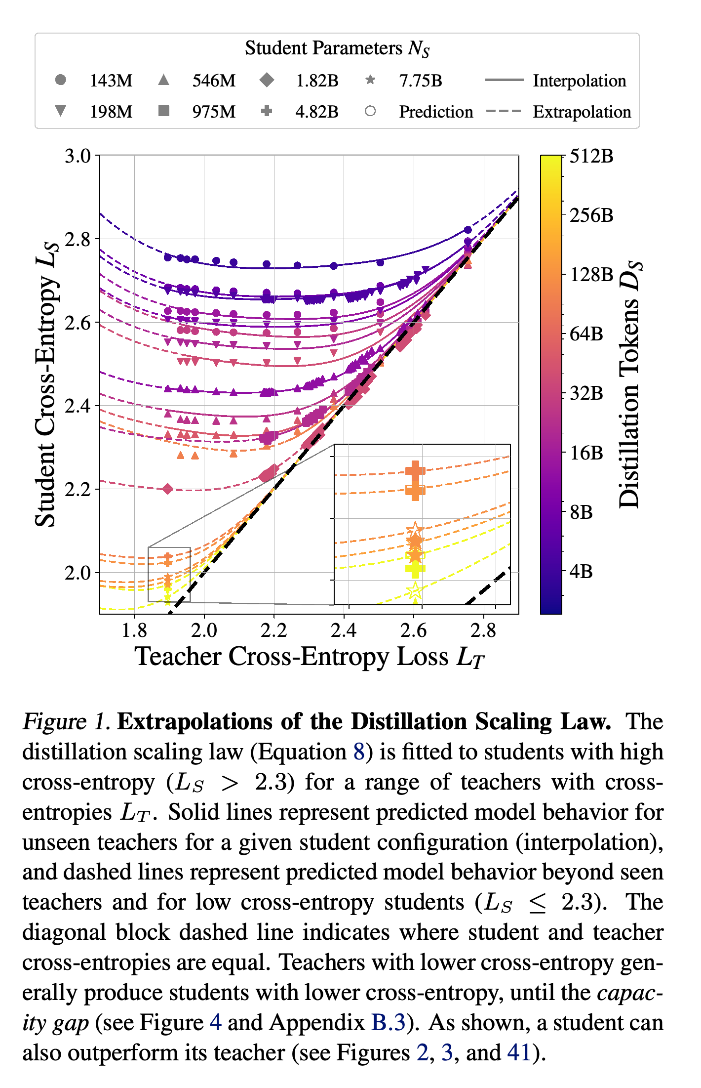
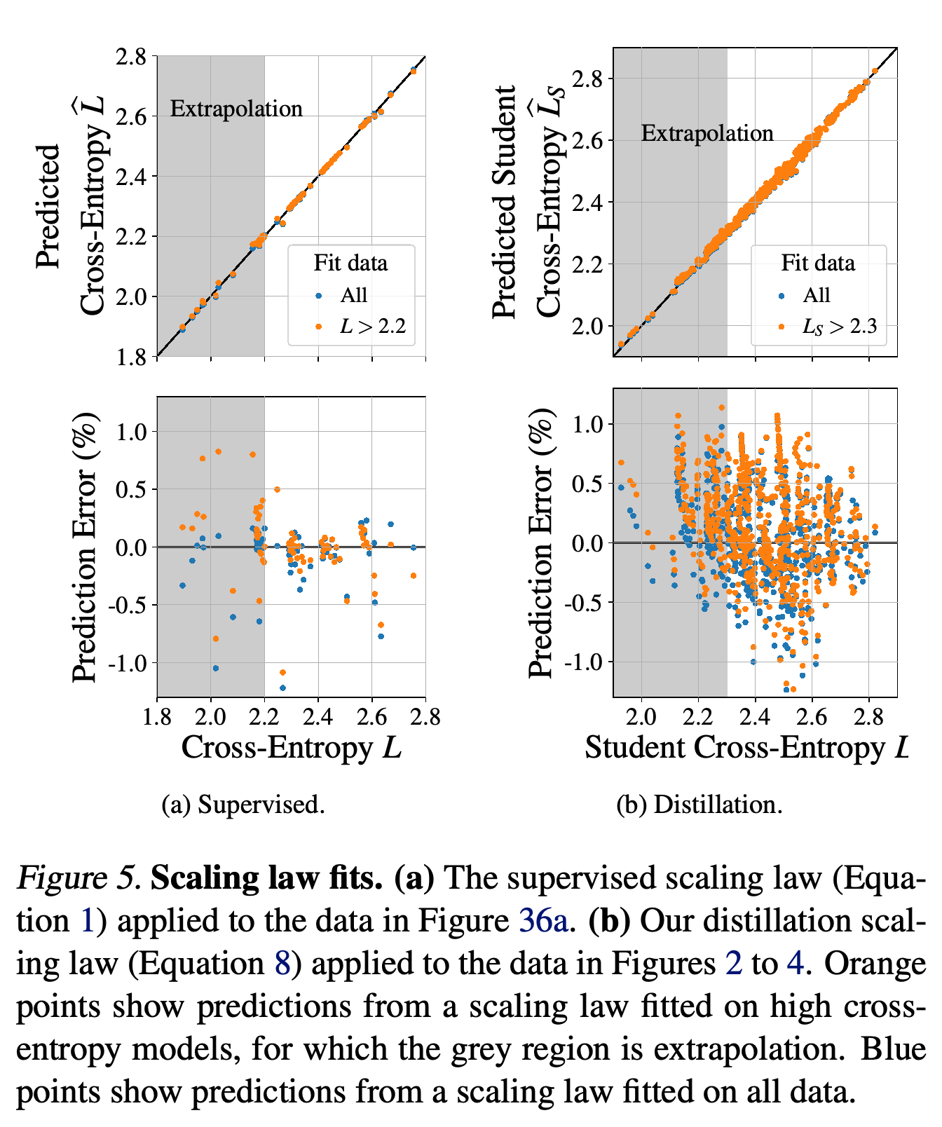
Predictions fitted to students with L_S > 2.3 track lower-loss students as well as unseen teacher configurations. The curved relationships show that improving teacher loss helps only up to a student-dependent optimum, linking the extrapolation test to capacity-gap behavior.
2. Background
The supervised baseline is Equation 1: \(L(N,D)=E+\left(\frac{A}{N^\alpha}+\frac{B}{D^\beta}\right)^\gamma\), where N counts non-embedding parameters, D counts training tokens, and E represents irreducible error. The positive coefficients are estimated from training runs rather than assumed universal.
- Compute-optimal runs alone approximately hold the token-to-parameter ratio M = D/N constant, preventing independent identification of parameter and data effects.
- The experimental design therefore combines fixed-model runs with varied data and IsoFLOP profiles, which vary model size and training tokens while holding floating-point operation counts fixed.
3. Preliminaries
An autoregressive language model predicts each next token from preceding tokens; its logits are scores converted into vocabulary probabilities by softmax, an exponential normalization function. Supervised next-token prediction uses the observed token as its target, whereas distillation uses the teacher’s probability distribution.
- The distillation objective is equivalent to minimizing forward Kullback–Leibler divergence, a measure of discrepancy from the teacher distribution to the student distribution, abbreviated KL divergence below.
- Equation 7 combines supervised loss and distillation loss with mixing coefficient λ, plus a Z-loss regularizer that stabilizes training by penalizing the squared logarithm of the softmax normalizing sum.
- Temperature τ rescales teacher and student logits before computing the distillation loss, changing the concentration of their probability distributions.
4. Distillation Scaling Laws
The scaling-law construction proceeds through controlled experiments, selection of a functional form, coefficient fitting, and extrapolation checks. The target is student validation loss against actual data, rather than the loss measuring agreement with teacher outputs.
4.1. Experimental Setup
All main experiments use English C4 and transformer models with sequence length 4096, multi-headed attention, which combines several attention computations, and normalization before model sublayers using RMSNorm, a root-mean-square normalization method. Rotary Position Embedding encodes token position through rotations. A simplified Maximal Update Parameterization, µP, sets parameter scaling to support transferring learning-rate settings across model sizes.
- Teacher pretraining and student distillation use different splits from the same data distribution. Appendix I gives approximately 90B unique tokens per split, so longer runs repeat data within their respective splits.
- The main scaling experiments use pure distillation, λ = 1, and temperature τ = 1. Appendix G examines these choices with mixing-coefficient and temperature sweeps.
- Parameter counts exclude embeddings unless otherwise stated, and teachers may be smaller or larger than their students.
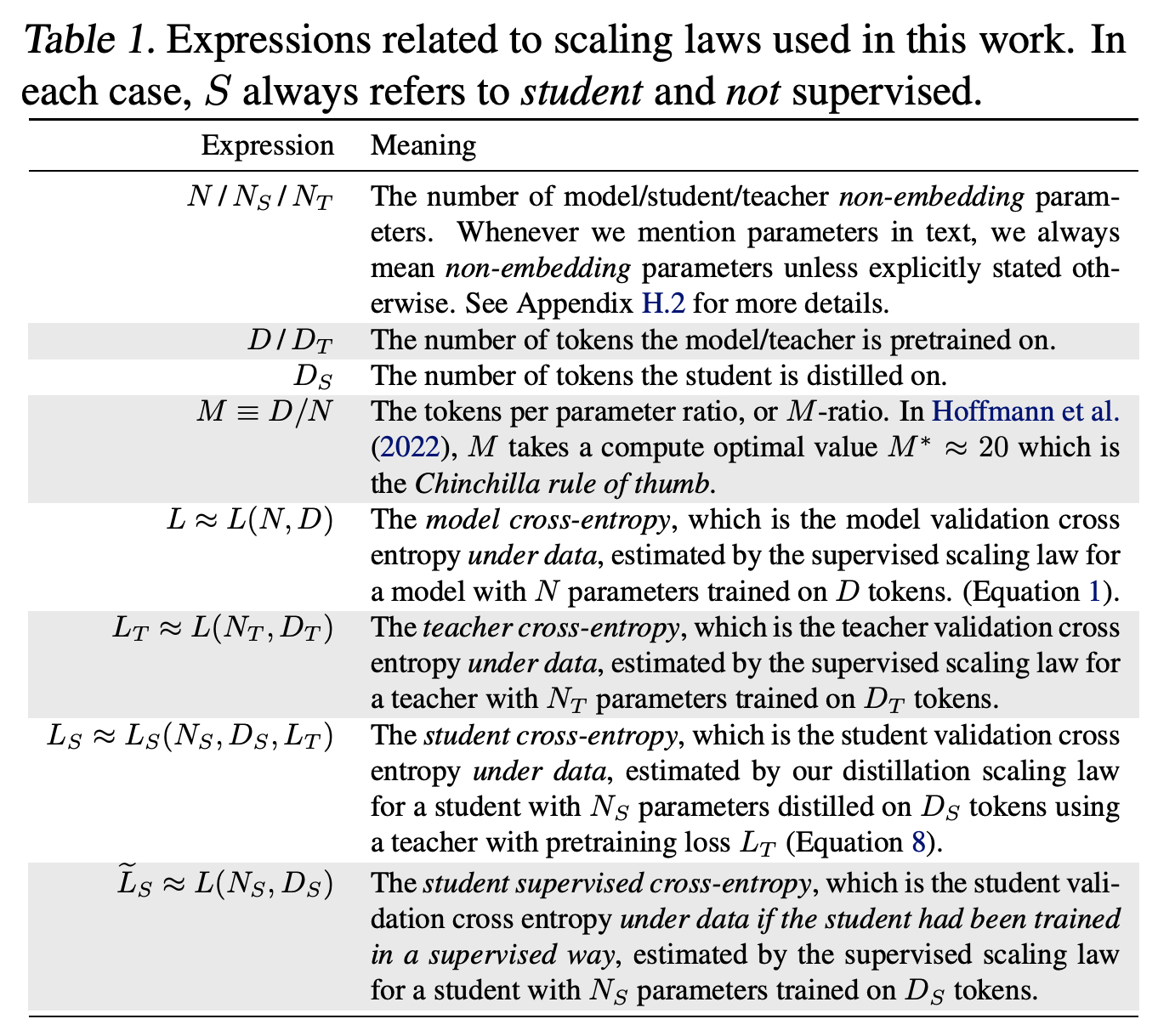
The notation distinguishes distilled student loss from the counterfactual loss of a supervised student with the same parameters and tokens. This distinction is necessary for interpreting the capacity transition and matched-resource comparisons.
4.2. Distillation Scaling Law Experiments
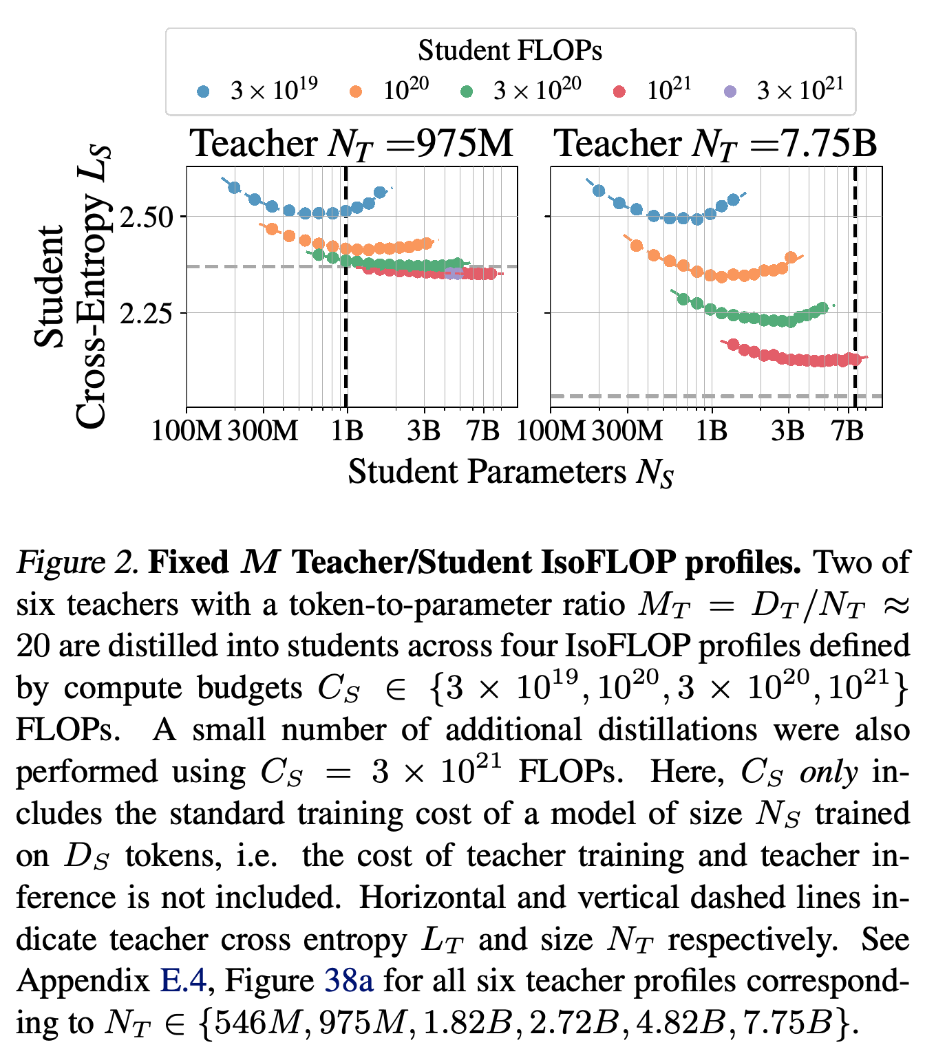
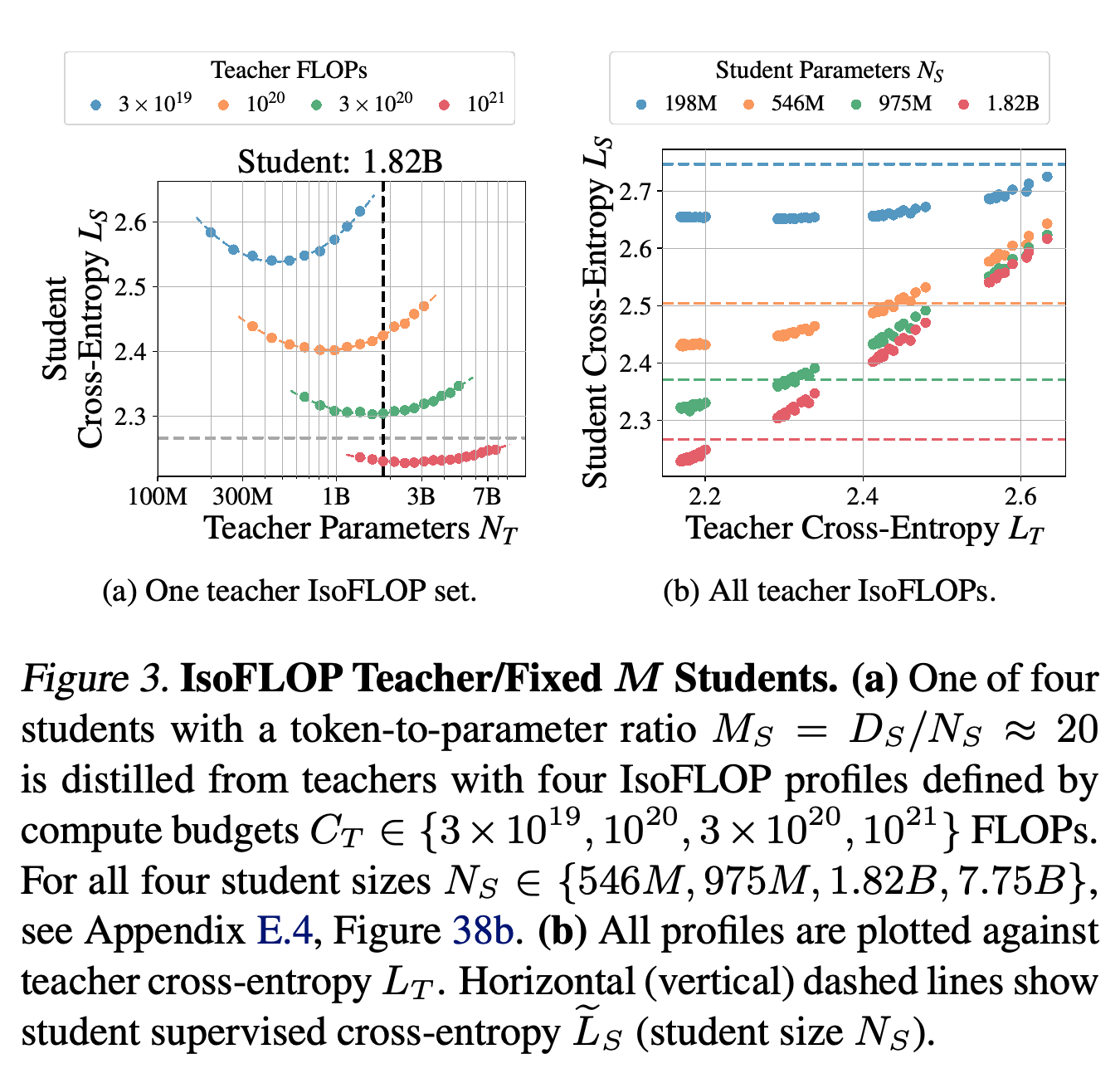
Three complementary protocols separate student-resource effects from teacher-quality effects: fixed-M teachers with student IsoFLOP profiles, teacher IsoFLOP profiles with fixed students, and fixed-M teacher–student combinations over varied student token budgets. Fixed-M denotes a constant token-to-parameter ratio, approximately 20 for the teachers. The principal compute profiles use 3 × 10^19, 10^20, 3 × 10^20, and 10^21 floating-point operations, with a smaller number of student runs at 3 × 10^21.
- Figure 2 shows that increasing student size at fixed student training compute eventually becomes counterproductive because fewer training tokens are available.
- Figure 3 shows that teachers with different parameter and token allocations produce a smooth student-loss relationship when indexed by teacher validation loss.
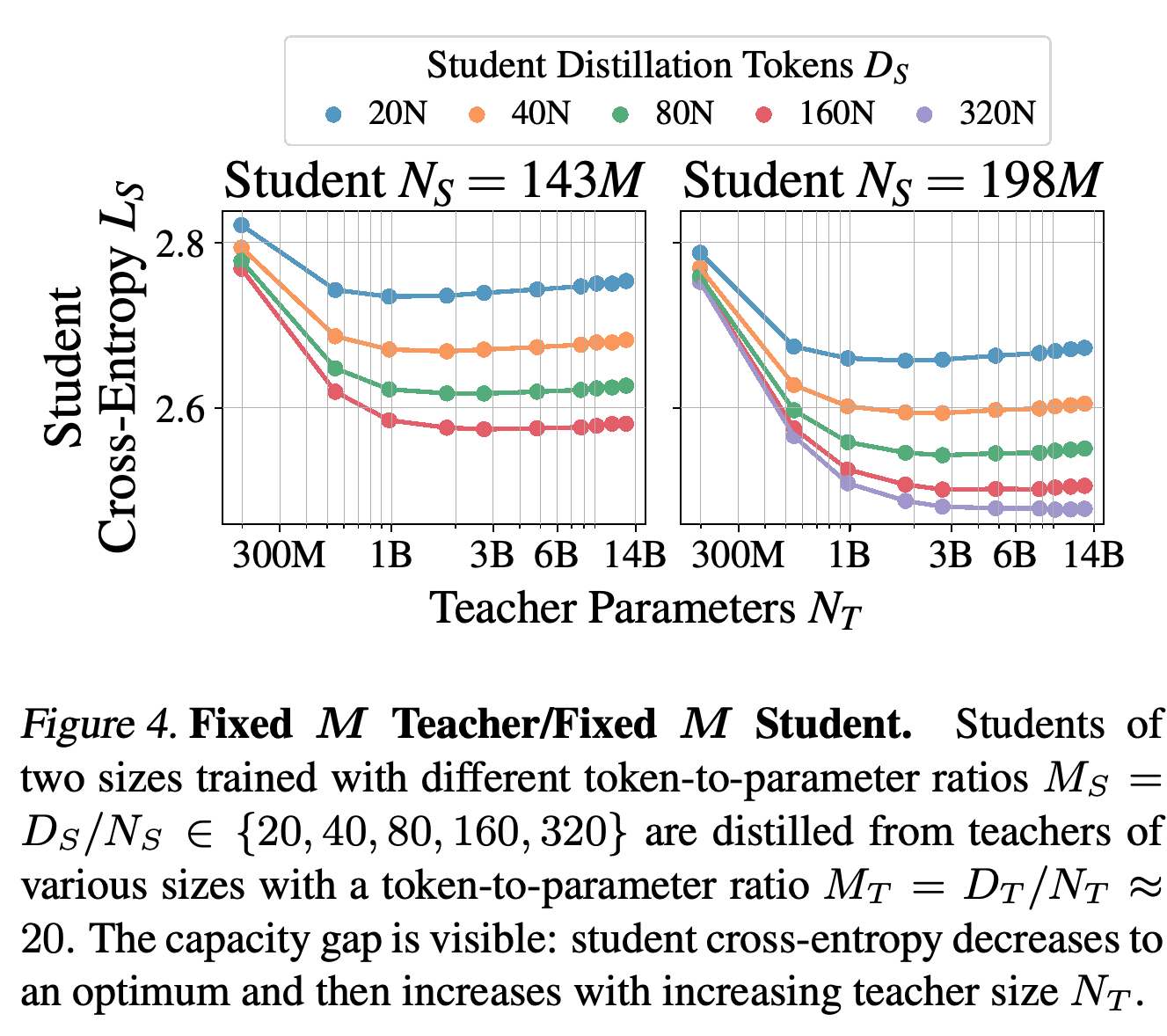
- Figure 4 demonstrates the capacity gap: at fixed student size and token budget, student loss first decreases and then increases as teachers become more capable. Teacher–student KL divergence increases even while teacher validation loss improves.
The fixed-compute profiles show why parameter count and training tokens must be varied together: increasing student size can eventually raise loss as the available token count falls. Teacher pretraining and inference costs are excluded, isolating student training allocation.
Teacher-size sweeps vary with teacher training compute, but plotting student loss against teacher validation loss produces smooth relationships for each student configuration. This supports replacing separate teacher-size and teacher-token inputs with teacher loss within the studied setup.
For the 143M and 198M students, larger fixed-M teachers first reduce student loss and then increase it. Additional student tokens lower the curves but do not eliminate the observed teacher-quality optimum.
4.3. Distillation Scaling Law Functional Form
Equation 8 combines a power law in student parameters and tokens with a broken power law, a smooth transition between two power-law regimes, in teacher loss. It is designed to capture teacher matching by an infinitely capable student, ineffective learning from a random teacher, and degradation when the teacher becomes too capable for the student.
- Using the primed coefficient notation restated in Appendix F.2, the functional form is L_S(N_S,D_S,L_T) = L_T + L_T^(−c_0)[1 + (L_T/(ṼL_S d_1))^(1/f_1)]^(−c_1 f_1)(A′/N_S^α′ + B′/D_S^β′)^γ′, where ṼL_S = L(N_S,D_S) is the corresponding supervised student loss.
- The transition depends on relative learning ability through L_T/ṼL_S, with transition parameter d_1. This makes teacher quality relative to student capability more informative than a teacher-to-student parameter ratio alone.
4.4. Distillation Scaling Law Parametric Fit
The authors fit the supervised law to teacher runs and the distillation law to the student experiments, reporting approximately 1% or less relative prediction error. Figure 5 tests extrapolation by fitting only weaker models: supervised models with L > 2.2 and distilled students with L_S > 2.3.
- The restricted fits predict lower-loss models with similar accuracy over the tested range, providing evidence beyond interpolation among fitted models.
- A separate numerical check finds approximate agreement between supervised and optimally distilled infinite-data limits for fixed model sizes. This comparison depends on the fitted coefficients and an imposed limiting condition; it is not an observation of infinite-data training.
The restricted-data fits remain close to measured losses in the shaded extrapolation regions. The relative-error panels provide the evidence behind the reported approximately 1% predictive accuracy over the evaluated models.
5. Distillation Scaling Law Applications
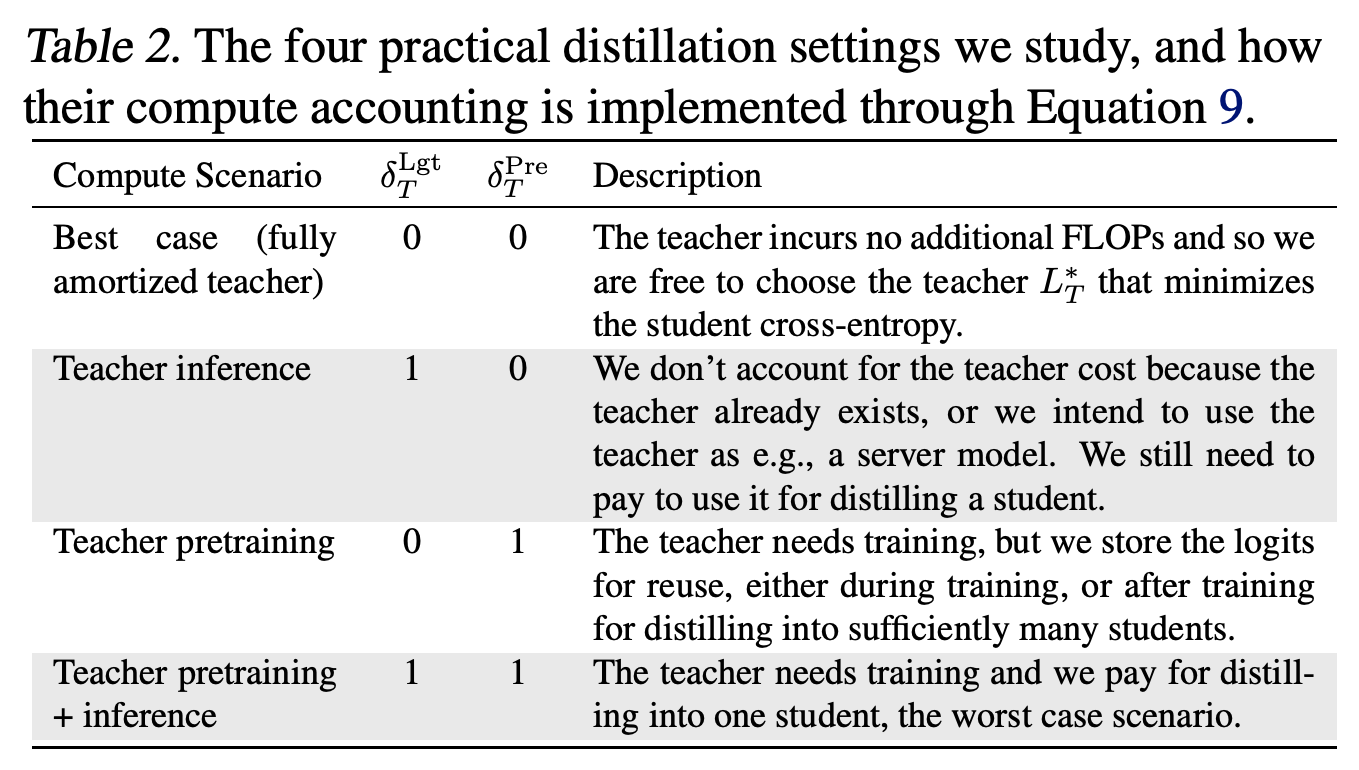
Equation 9 accounts separately for student training, teacher inference to produce logits, and teacher pretraining: FLOPs ≈ 3F(N_S)D_S + F(N_T)(δ_T^Lgt D_S + 3δ_T^Pre D_T). Here FLOPs counts floating-point operations, F(N) is forward floating-point operations per token, and the two δ terms determine whether teacher inference and pretraining are charged to the budget.
- Table 2 defines four settings: both teacher costs excluded, teacher inference included, teacher pretraining included, and both teacher costs included.
- The usual F(N) ≈ 2N approximation undercounts important context and vocabulary costs for small models. The paper instead derives a correction for architectures with a fixed ratio of model width to layer count.
The two teacher-cost terms determine which resources the comparison charges to a student. An existing teacher still incurs inference cost unless its outputs are already available or that cost is shared; training a teacher solely for one student includes both terms.
5.1. Fixed Tokens or Compute (Best Case)
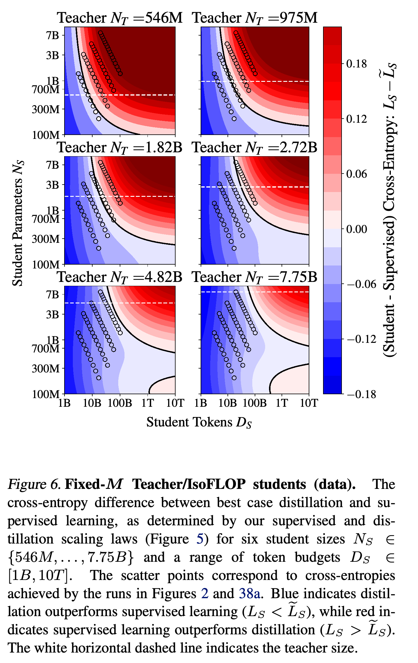
With teacher costs excluded, distillation can outperform a supervised student using the same student resources when token or compute budgets are modest and the teacher is suitable. For a fixed teacher, increasing student resources eventually favors supervised training unless the teacher is optimally chosen. Optimally chosen distillation approaches the same limiting performance as supervised training.
- Figure 6 maps the difference between distilled and supervised loss over student sizes and token budgets from 1B to 10T, with observed runs overlaid on fitted contours.
- The comparison concerns efficiency relative to supervised training. Longer distillation may still improve a student’s absolute performance while becoming less efficient than direct training.
Blue regions identify student configurations where distillation beats direct training, while red regions favor the supervised baseline. Increasing student token budgets can cross this boundary even when the same teacher is retained.
5.2. Fixed Tokens or Compute (Teacher Inference)
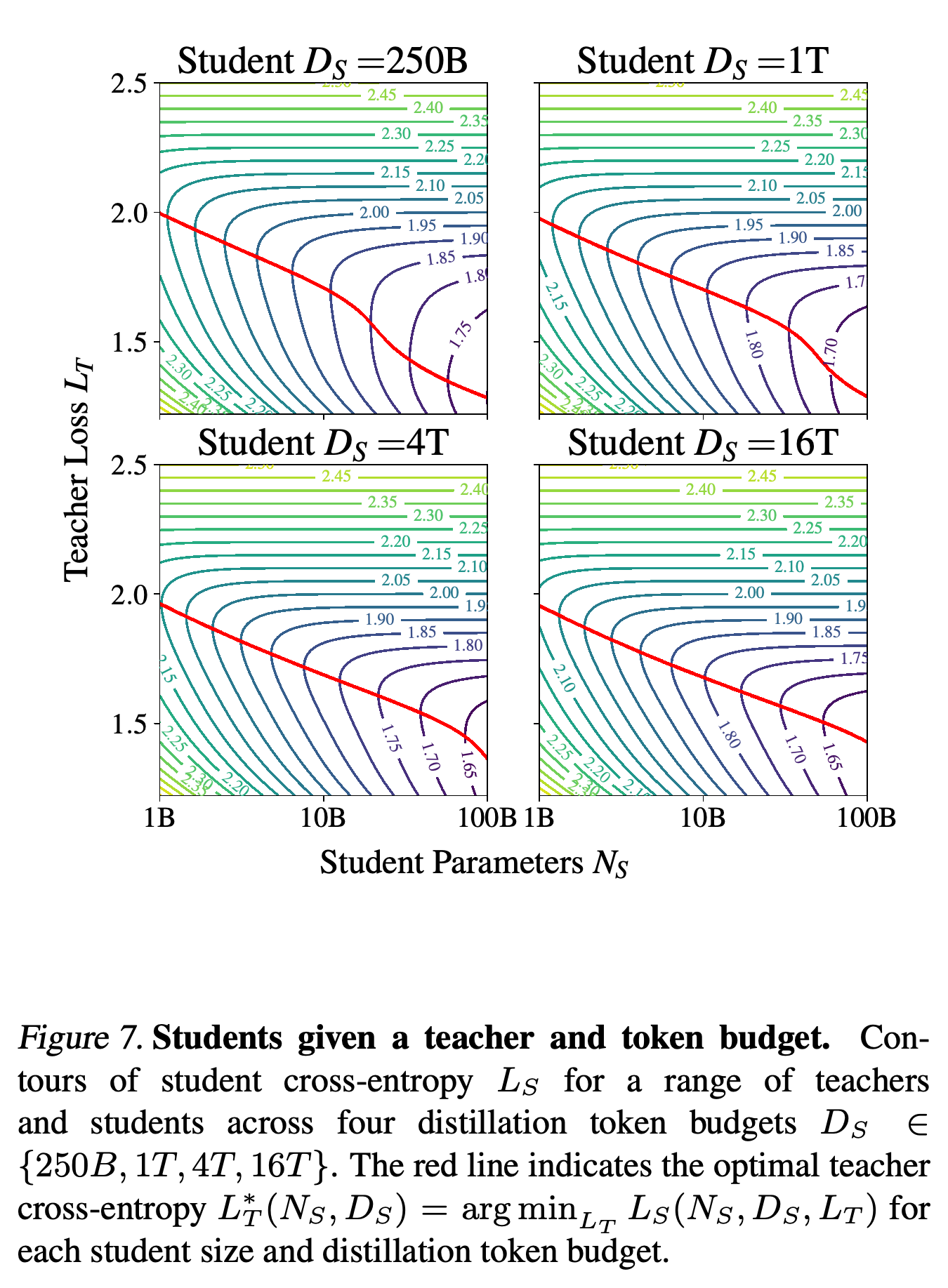
When selecting among existing teachers, teacher quality and teacher inference cost create a trade-off: a larger teacher may improve the learning signal while reducing the number of student tokens affordable under fixed compute. Under a fixed token budget, the optimal teacher loss decreases approximately as a power law with student size, with a sharper change near the point where optimal teacher loss matches the corresponding supervised student loss.
- Figure 7 evaluates token budgets of 250B, 1T, 4T, and 16T and identifies the teacher loss minimizing student loss for each student size.
- The relevant quality variable is teacher validation loss. Teacher parameter count additionally matters when inference costs enter the budget.
The red minimizing curves show that teacher selection depends on student size and token budget. Selecting the lowest-loss teacher without regard to the student can move away from the optimum because of the capacity gap.
5.3. Compute Optimal Distillation
For a prescribed student size, Equation 10 minimizes predicted student loss over student tokens, teacher size, and teacher training tokens subject to a compute budget. The numerical solution uses Sequential Least SQuares Programming, a constrained optimization method, implemented in SciPy.
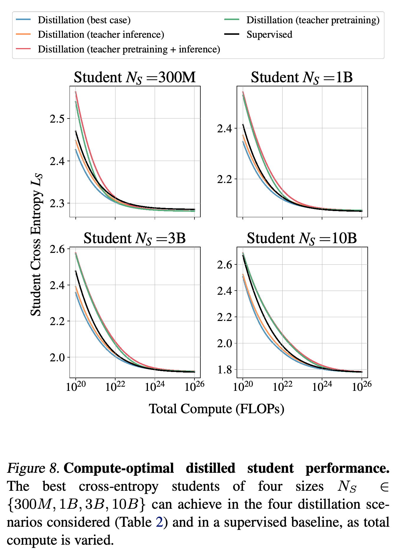
- Figure 8 shows that excluding teacher pretraining permits distillation gains at lower compute, while supervised training catches up at a compute level that increases with student size.
- Charging teacher pretraining to a single student produces higher predicted loss than direct supervised training, with losses approaching one another at very large budgets. Reusing a teacher or sharing its costs across multiple students can change this accounting.
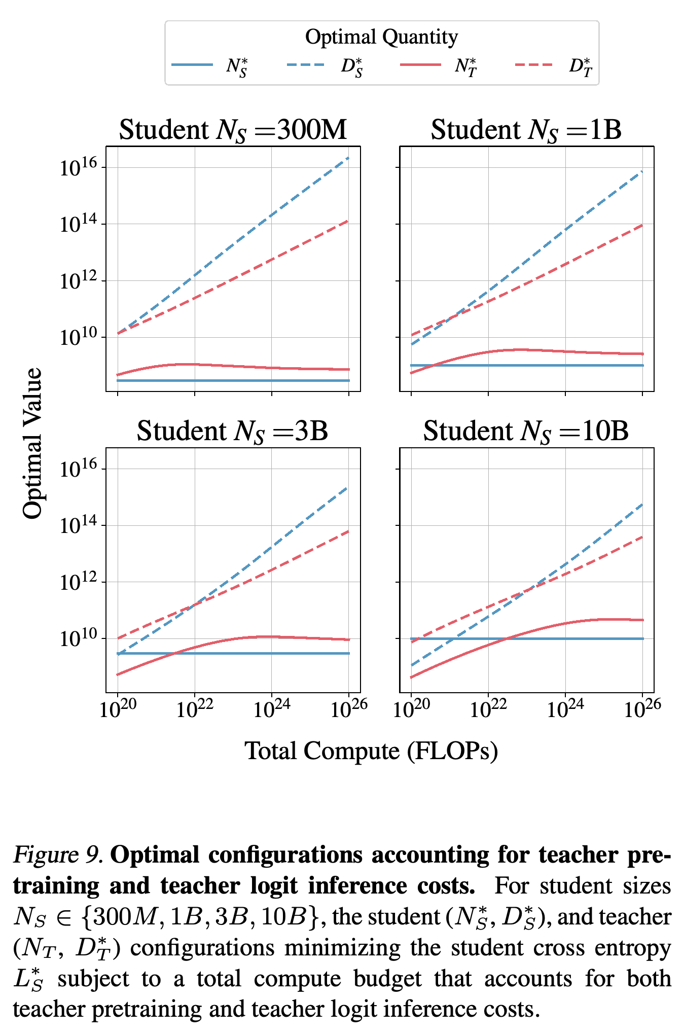
- When both teacher costs count, Figure 9 predicts that student tokens grow faster than teacher tokens. Teacher size initially increases and then levels off or declines slightly, making additional teacher training more economical than continually increasing teacher size.
The curves distinguish gains available when teacher pretraining is excluded from comparisons that charge for building the teacher. The compute range benefiting from distillation expands with student size, while supervised training approaches the same limiting loss at larger budgets.
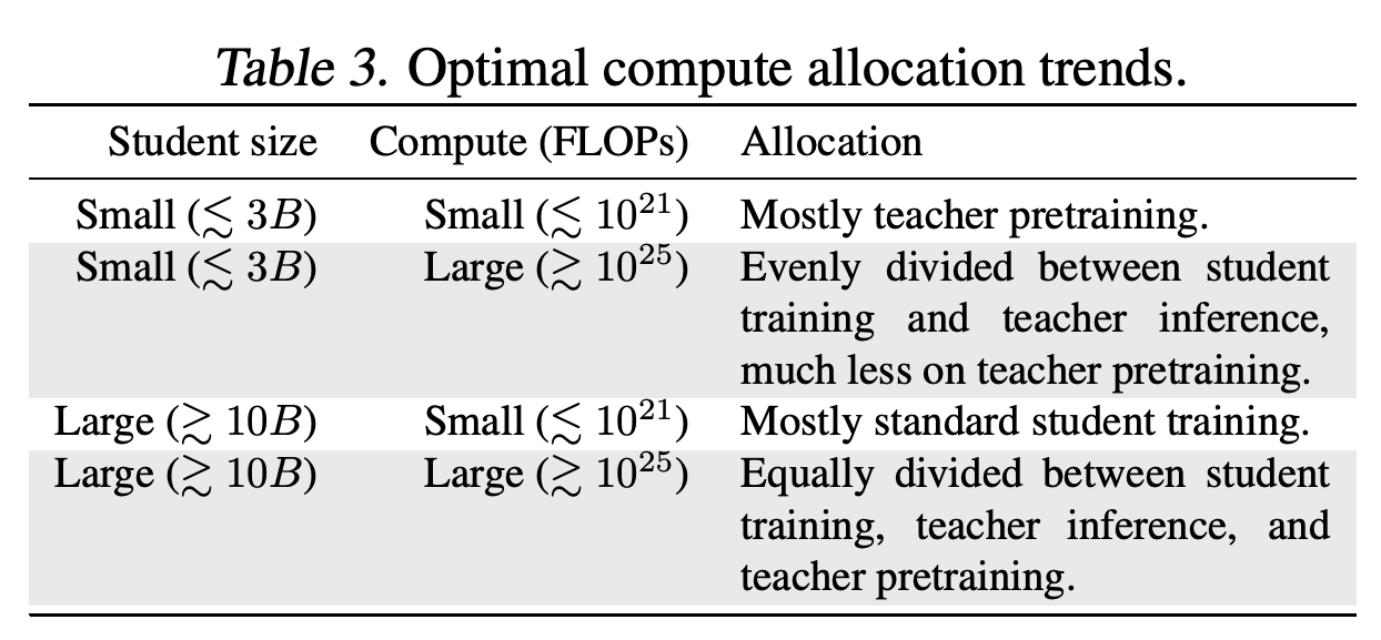
For the setting including both teacher costs, the table assigns mostly teacher pretraining to small students at small budgets and mostly student training to large students at small budgets. At large budgets it lists an approximately even student-training and teacher-inference split for small students, with little teacher pretraining, and roughly equal allocations to all three components for large students. These are qualitative regime summaries rather than exact allocation rules.
Student token counts rise faster than teacher token counts while teacher parameter counts flatten or decline slightly after an initial increase. These fitted-law optima explain the shift toward further training of a moderately sized teacher when repeated teacher inference becomes costly.
6. Conclusion
The paper provides a resource-allocation model that makes teacher selection and cost accounting explicit. Distillation can be more efficient below a student-size-dependent resource threshold when teacher costs are already paid or sufficiently shared. Training a teacher exclusively for one student generally loses to direct supervised pretraining in the paper’s comparisons.
Impact Statement
The Impact Statement identifies potential benefits from reducing inference costs, avoiding unnecessary training experiments, and making capable small models more accessible. These are proposed consequences of improved training allocation, rather than measured deployment or carbon-emissions results.
- The authors also identify teacher-bias inheritance and cheaper malicious use, including targeted misinformation, as potential negative consequences of efficient distilled models.
Appendix
- A. Limitations restricts the evidence to language modeling on English C4, transformer teacher–student architectures, and training splits drawn from the same distribution. Longer runs repeat data, reasoning evaluations are limited, and the fitted coefficients are architecture- and dataset-specific. The law is empirical rather than derived from first principles, and its applicability to Sequence-Level Knowledge Distillation, which trains on generated token sequences, remains unverified.
- B. Extended background reviews related evidence. B.1. Knowledge Distillation distinguishes fidelity, agreement with the teacher’s predictive distribution, from student generalization and discusses why longer distillation can improve absolute performance while losing efficiency against a matched supervised baseline. B.2. Neural Scaling Laws relates the study to resource scaling and transfer between data distributions, while B.3. The Knowledge Distillation Capacity Gap reviews explanations and interventions and argues that teacher loss captures effects of both teacher size and training duration.
- C. Teacher Student Capacity Gaps supplies two controlled demonstrations. C.1. Kernel Regression, function fitting in a space spanned by basis functions, uses C.1.1. SETUP and C.1.2. DISTILLING THE TEACHER to derive optimal teacher and student functions with finite basis sets and norm constraints under infinite data. C.1.3. U-SHAPE IN THE STUDENT ERROR establishes non-increasing student error while teacher capacity m is below student capacity n, followed by non-decreasing error for m ≥ n: additional teacher basis functions can reduce the teacher’s allocation to components the student can represent. C.2. MLPs on the Mapping Problem, including C.2.1. PROBLEM DEFINITION and C.2.2. EXPERIMENTAL FINDINGS, tests a synthetic task combining direct position identification and contextual remapping. A multi-layer perceptron, or MLP, is a feed-forward network; here it has two equally wide hidden layers and is trained using Adam, an adaptive gradient optimizer, peak learning rate 3 × 10^−4, batch size 512, and non-repeated samples. A width-256 student first improves and then deteriorates as teacher width or teacher training duration increases; figures report the 25% and 75% values across four trials.
- D. Distillation scaling law applications (additional results) expands the resource comparisons. D.1. Experimental differences resolving the apparent contradiction with patient teachers explains differences in data access and supervised baselines; D.2. Fixed tokens or compute (best case) separates teacher-resource gains from eventual student saturation. D.3. Fixed size or compute (teacher inference) shows that stronger teachers need not be preferable when their inference cost leaves too few student tokens. D.4. Compute optimal distillation and D.4.1. SETUP allow numerical teacher sizes and token counts in [1M,100P], with P denoting 10^15, deliberately extending beyond available data resources; D.4.2. CROSS-ENTROPY compares eight student sizes. D.4.3. DISTILLATION (BEST CASE) leaves teacher size and training tokens non-unique at a chosen teacher loss; D.4.4. DISTILLATION (TEACHER INFERENCE) favors overtrained teachers and drives teacher tokens to the optimization ceiling of 10^17. D.4.5. DISTILLATION (TEACHER PRETRAINING) favors supervised-compute-optimal teachers, while D.4.6. DISTILLATION (TEACHER PRETRAINING + INFERENCE) shifts from compute-optimal teachers toward overtrained teachers as student-token costs grow. D.4.7. OPTIMAL TEACHER TRAINING AND STUDENT DISTILLATION TOKENS finds similar growth rates for student tokens across scenarios, with scenario-dependent offsets, while teacher tokens follow different trajectories; D.4.8. OPTIMAL TEACHER SIZE likewise compares teacher-size trajectories across cost scenarios. D.5. Compute and data efficiency gains for distillation compared to supervised learning expresses distillation compute and tokens relative to the supervised resources required for the same student loss, counting teacher tokens only when teacher pretraining is charged. The authors suggest beginning with distillation and switching to supervised training near saturation, but leave that strategy untested.
- E. Additional Results begins with E.1. Downstream evaluations: supervised and distilled models follow similar relationships between validation loss and standard English task performance. ARC Easy and ARC Challenge, science-question benchmarks, HellaSwag, a sentence-completion benchmark, Piqa, a physical-commonsense benchmark, Sciq, a science-question benchmark, WinoGrande, a pronoun-resolution benchmark, and Lambada OpenAI, a contextual word-prediction benchmark, use zero-shot evaluation, meaning no demonstration examples; TriviaQA and WebQS, question-answering benchmarks, use one example. GSM8K, a mathematics word-problem benchmark, uses eight examples with intermediate reasoning demonstrations, and MMLU, a multitask knowledge benchmark, uses five examples, but most models perform near random on these latter evaluations, limiting conclusions about reasoning. E.2. Teachers used in distillation documents fixed-M, 512B-token, and IsoFLOP supervised teacher runs; E.3. Fixed-M teacher/fixed-M students and the capacity gap shows increasing teacher–student divergence. E.4. Full distillation scaling law IsoFLOP profiles and E.5. Distillation scaling law IsoFLOP optima provide complete resource sweeps and minima, while E.6. Distillation with infinite data checks approximate numerical agreement between optimally distilled and supervised limiting losses under a condition imposed on the fitted law. E.7. Weak-to-strong generalization, meaning a student outperforming its teacher, places this behavior in the finite-data regime in the examined setting and observes convergence toward teacher behavior with sufficiently extensive distillation. E.8. Model calibration measures agreement between predicted confidence and observed accuracy using Expected Calibration Error, ECE, over 21 bins, and introduces a distributional variant comparing teacher and student probabilities. E.8.1. TEACHERS shows generally low error, so teacher miscalibration alone cannot explain the capacity gap. E.8.2. 198M STUDENTS TRAINED ON 20N TOKENS and E.8.3. 198M STUDENTS TRAINED ON 128B TOKENS show that full-distribution training preserves calibration against actual data much better than training only on the teacher’s most probable token; longer training improves calibration when the training target and evaluated quantity agree.
- F. Scaling coefficients, comprising F.1. Supervised scaling law coefficient estimation, F.2. Distillation scaling law coefficient estimation, and F.3. Scaling law coefficients parameteric fit, describes log-space fitting with Huber loss, which combines quadratic and linear penalties, threshold δ = 10^−4, and multiple L-BFGS-B initializations, a bounded numerical optimization procedure. Table 6 reports 73 supervised and 697 distillation fitting runs, with 90% confidence intervals from 4096 bootstrap resamples, repeated samples drawn from the fitting data. The distillation estimates include α′ = 0.321, β′ = 0.637, γ′ = 0.764, c_0 = 2.549, c_1 = 522.6, f_1 = 0.090, and d_1 = 1.315.
- G. Distilling language models in practice tests implementation choices: G.1. Mixing coefficient (λ) sensitivity analysis finds broadly flat student loss for λ > 0.5 except with weak teachers, G.2. Temperature (τ) sensitivity analysis finds τ = 1 best over τ ∈ [0.5,10], and G.3. Learning rate (η) sensitivity analysis, verification of µP for distillation supports η = 0.01 over sweeps in [0.001,0.1] for the tested configurations. G.4. Distribution truncation methods: Top-k and Top-p sensitivity retains either the k largest teacher probabilities or a smallest set reaching cumulative probability p; this degrades pure distillation, but k = 128 with λ = 0.7 stays within 0.01 nats of full-distribution performance, where a nat is a natural-log unit of loss. G.5. Forward and reverse KL divergence reverses the teacher and student arguments of the discrepancy measure and reports losses of 2.42 and 2.70, respectively, for a 1.82B teacher and 546M student, a 0.28-nat advantage for forward KL in that comparison.
- H. Parameters and Floating Operation Estimation, through H.1. Alternative approximation for FLOPs per token as a function of N, H.2. Model parameters, and H.3. FLOPs per token, retains attention-context and vocabulary-projection costs omitted by the simple 2N estimate and accounts for efficient causal attention, which excludes future tokens. Equation 69 gives C_Forward = 2N(1 + σ_1 n_ctx/N^(1/3) + σ_2 n_vocab/N^(2/3)), where n_ctx is context length, n_vocab is vocabulary size, and σ_1 and σ_2 depend on architecture ratios. Table 13 illustrates the consequence: for the 143M model, the 2N estimate has −36.10% relative error, while the corrected estimate has −0.34%.
- I. Model architecture specifies AXLearn, the training library, weight decay 10^−4, peak learning rate 1e−2, gradient global-norm limit 1.0, 2000 warmup steps, cosine learning-rate decay, and Z-loss coefficient 10^−4. Models use a width-to-layer-count ratio of 128, feed-forward ratio 8/3, and rotary-embedding base frequency 500k.
- J. Contributions assigns experimental, fitting, theoretical, evaluation, and ablation work to the authors and states that all authors contributed to writing, experiment design, and discussion.
Brief Thoughts
The explicit separation of teacher quality from teacher cost makes the results useful for experiment planning: Figures 3–5 support loss-based prediction, while Table 2 and Figure 8 show how cost accounting changes the comparison with supervised training. The tested extrapolations support planning within a related experimental setting, but do not validate numerical optima far beyond the observed model and data ranges as deployment recipes.
The evidence is strongest for full-distribution pretraining distillation; generated-sequence distillation and reasoning remain outside the demonstrated scope. Some appendix details require care: E.8.3 names 128B tokens while its opening paragraph states approximately 512B, and D.5’s example attributed to pretraining + inference conflicts with its preceding comparison and plotted cost ratios. These inconsistencies leave the specific appendix quantities uncertain; the main-body comparisons consistently favor supervised training when a teacher’s full training cost is charged to one student.