Densing Law of LLMs | Summary

Contents

Summary
Highlights
1 Introduction
- 1.1 Key Findings
2 Density for Large Language Models
3 Density Evolution
4 Discussion
5 Limitations and Future Directions
6 Conclusion
Appendix
Brief Thoughts

This article explains the key points of Densing Law of LLMs.

2024-12-05 (arXiv)
Xiao, Chaojun, Cai, Jie, Zhao, Weilin, Zeng, Guoyang, Lin, Biyuan, Zhou, Jie, Zheng, Zhi, Han, Xu, Liu, Zhiyuan, Sun, Maosong.
Tsinghua University, ModelBest Inc.
Paper

Summary

Comparing large language models (LLMs) across parameter counts requires a measure that accounts for both task performance and model size. Across 29 open-source pretrained base models—models evaluated without subsequent instruction tuning or learning from preferences—the authors find that maximum capability density approximately doubles every three months under their five-benchmark evaluation and chosen reference setup. Capability density divides the reference-model parameter count needed to match a model’s performance by that model’s actual parameter count.
The method first fits parameter count and training-data size to conditional answer loss, which measures how well a model predicts answers given task inputs, then fits loss to benchmark performance. Inverting these relationships at a reference training budget of 1 trillion tokens yields an effective parameter count: the reference size needed to match the target score. The main analysis reports a maximum-density growth rate of A ≈ 0.0073 per day, a doubling time of approximately 95 days, and R² = 0.912, a measure of regression fit.
The contribution is a reference-dependent comparison of benchmark performance and parameter efficiency, together with an empirical account of the historical maximum-density frontier. Benchmark contamination, meaning exposure to test-like data during training, limited task coverage, and exclusion of subsequent training and variable inference computation restrict its interpretation. The trend does not establish a guaranteed replacement schedule or directly measure deployment costs.

Highlights

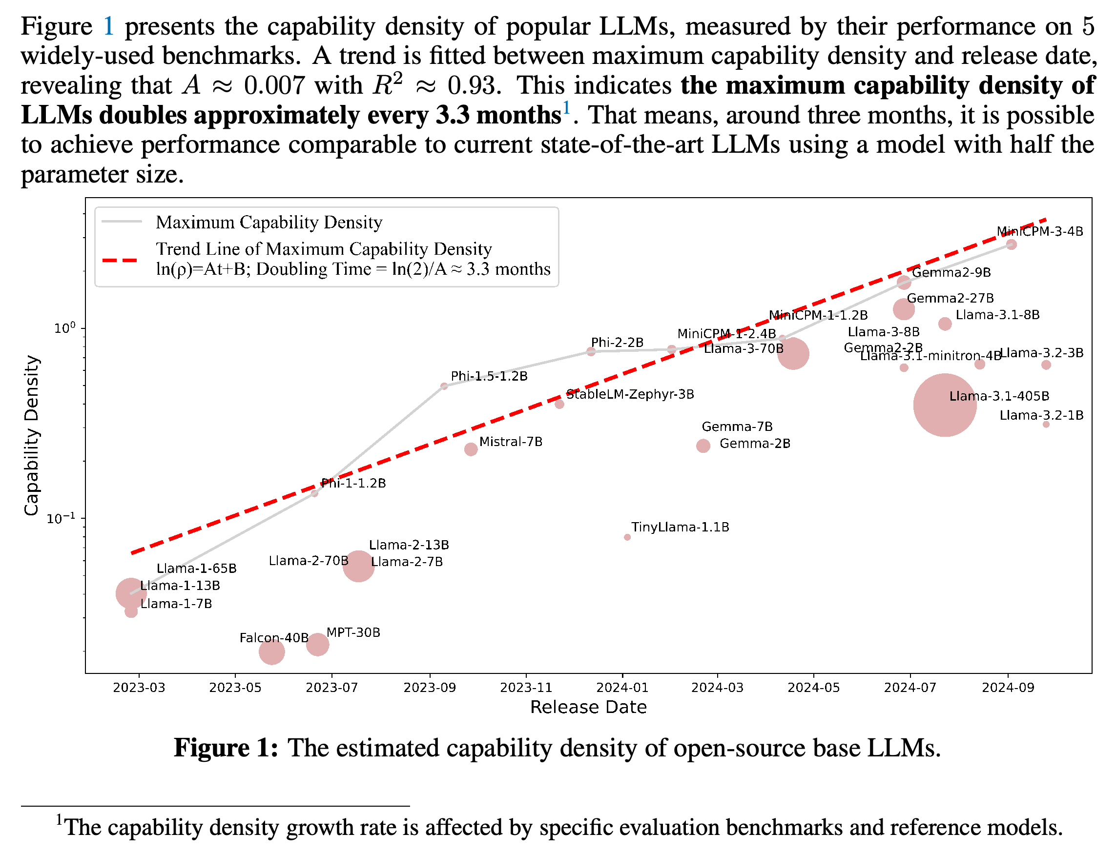
Highlights defines relative capability density using the minimum reference-model parameter count required to achieve equivalent performance. It states the Densing Law as $\ln(\rho_{\max})=At+B$, where ρ_max is maximum density at time t and A and B are fitted coefficients, and reports A ≈ 0.007, R² ≈ 0.93, and a doubling time of approximately 3.3 months. Its footnote explicitly states that the growth rate depends on the evaluation benchmarks and reference models.

Estimated capability density of open-source base language models by release date, with the maximum-density envelope and its fitted exponential trend.

1 Introduction

The introduction connects increasing parameter and data scales with improved performance, while inference—the computation used to produce model outputs—creates costs that motivate compact models for applications such as smartphone deployment. Longer reasoning outputs add to this demand. Scaling laws, fitted relationships between model scale and performance or loss, motivate a reference-based comparison of performance and parameter efficiency.

1.1 Key Findings

The key finding concerns the maximum-density frontier across 29 open-source pretrained base models. As a concrete comparison, the authors report that MiniCPM-1-2.4B, released on February 1st, 2024, matches or exceeds Mistral-7B, released on September 27th, 2023, using approximately 35% as many parameters after four months.

The authors discuss five implications: declining inference costs at equivalent performance, combined algorithmic and hardware progress, faster density growth after ChatGPT’s release, compression that can reduce density, and training that prioritizes density.
Pruning removes model components, while distillation trains a smaller model using a larger model. The paper’s compression comparisons show that these procedures do not consistently increase capability density.

2 Density for Large Language Models

Density for Large Language Models formalizes the ratio of effective parameter size to actual parameter size. Its construction requires estimating how a chosen reference training setup maps parameter count to downstream performance, meaning scores on the evaluated tasks.

2.1 Overall Framework and Definition

For a target model M with N_M parameters and score S_M, the reference relationship S = f(N) defines effective size as N̂(S_M) = f⁻¹(S_M). Capability density is ρ(M) = N̂(S_M)/N_M, so density above one means that the reference setup requires more parameters to match the target model.

The authors decompose f into parameter-to-loss estimation and loss-to-performance estimation. Small reference models supply the first relationship, while better-trained models supply the second because small scaling experiments often achieve only chance-level task scores.

2.2 Loss Estimation

Loss Estimation models conditional answer loss, L = −log P(answer | instruction), using $\mathcal{L}=aN^{-\alpha}+bD^{-\beta}$, where N is parameter count, D is training-token count, and a, α, b, and β are fitted coefficients. This measures answer likelihood given task inputs rather than the likelihood of complete input-output sequences.

For multiple-choice tasks, inputs contain the question and all options, and loss is computed on an analysis followed by the correct answer label. For complex problems, the scored output includes reasoning steps and the correct answer.
For these task types, GPT-4o generates reasoning steps for all test instances because most datasets do not provide them. These generated explanations form part of the loss-estimation procedure.

2.3 Performance Estimation

Performance Estimation fits S = c/[1 + e^(−γ(L − l))] + d, a sigmoid, or S-shaped, relationship between conditional loss and task score. The fitted coefficients c, γ, l, and d determine the curve’s scale, transition, and limiting score levels.

Well-trained open-source models extend the observed performance range beyond that of the small loss-estimation models. The authors motivate the sigmoid using bounded benchmark scores, chance-level performance at high loss, and an upper plateau at low loss.

2.4 Density

Density inverts the two fitted functions while fixing reference training data to D = D₀ = 1T tokens, where 1T means 1 trillion. The resulting effective parameter size describes the reference model trained on that token budget that would match the target score; it does not specify the target model’s own training budget.

Equation (4) gives L̂(S_M) = l − (1/γ) ln[c/(S_M − d) − 1] and N̂(S_M) = [(L̂(S_M) − bD₀^(−β))/a]^(−1/α). Dividing this effective size by actual size produces density.
A model that achieves better performance with the same parameter count receives higher density under the fitted reference relationship.

3 Density Evolution

Density Evolution applies the metric to model releases over time. Its subsections establish the evaluation protocol, check the loss-to-performance estimator, and fit the historical maximum-density frontier.

3.1 Evaluation Settings

The five benchmarks are MMLU for English knowledge-intensive tasks, BBH for challenging logical reasoning, MATH for mathematical reasoning, and HumanEval and MBPP for coding. Their respective evaluation conditions are 5-shot, 3-shot, 4-shot, 0-shot, and 3-shot, where shot counts specify the number of demonstrations in the prompt. BBH, MATH, and MBPP use chain-of-thought prompting, which provides intermediate reasoning steps.

The small reference models use the MiniCPM-3-4B training corpus. Their learning-rate schedule follows warmup, stable-rate, and decay phases.
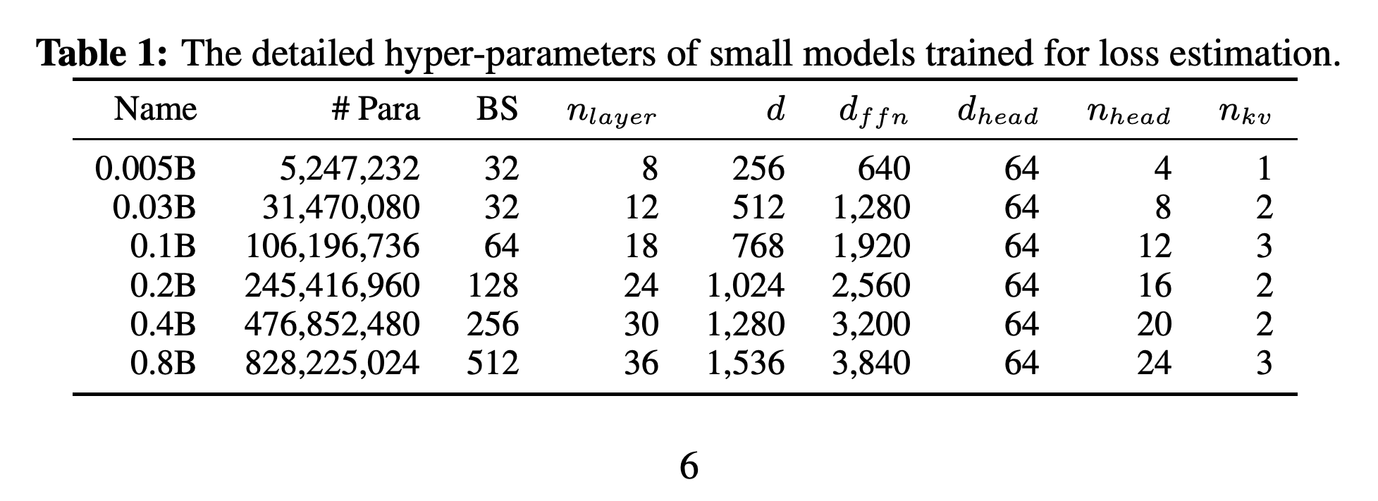
Table 1 lists six reference sizes from 5,247,232 to 828,225,024 parameters. Training budgets are {10, 15, 20, 30, 40, 60} × N tokens, where N is parameter count.
Loss-to-performance fitting uses MiniCPM-3 models and intermediate training checkpoints ranging from 0.5 billion to tens of billions of parameters. They share the reference models’ vocabulary, the set of tokens available to the models.
The temporal analysis prioritizes scores from model technical reports and covers pretrained base models without subsequent supervised fine-tuning, training on labeled examples, or preference learning. The authors acknowledge that benchmark-like data can still occur during pretraining.

Parameter counts, batch sizes, layer counts, hidden and feedforward dimensions, and attention-head configurations of the small loss-estimation models.

3.2 Loss and Performance Estimation Results

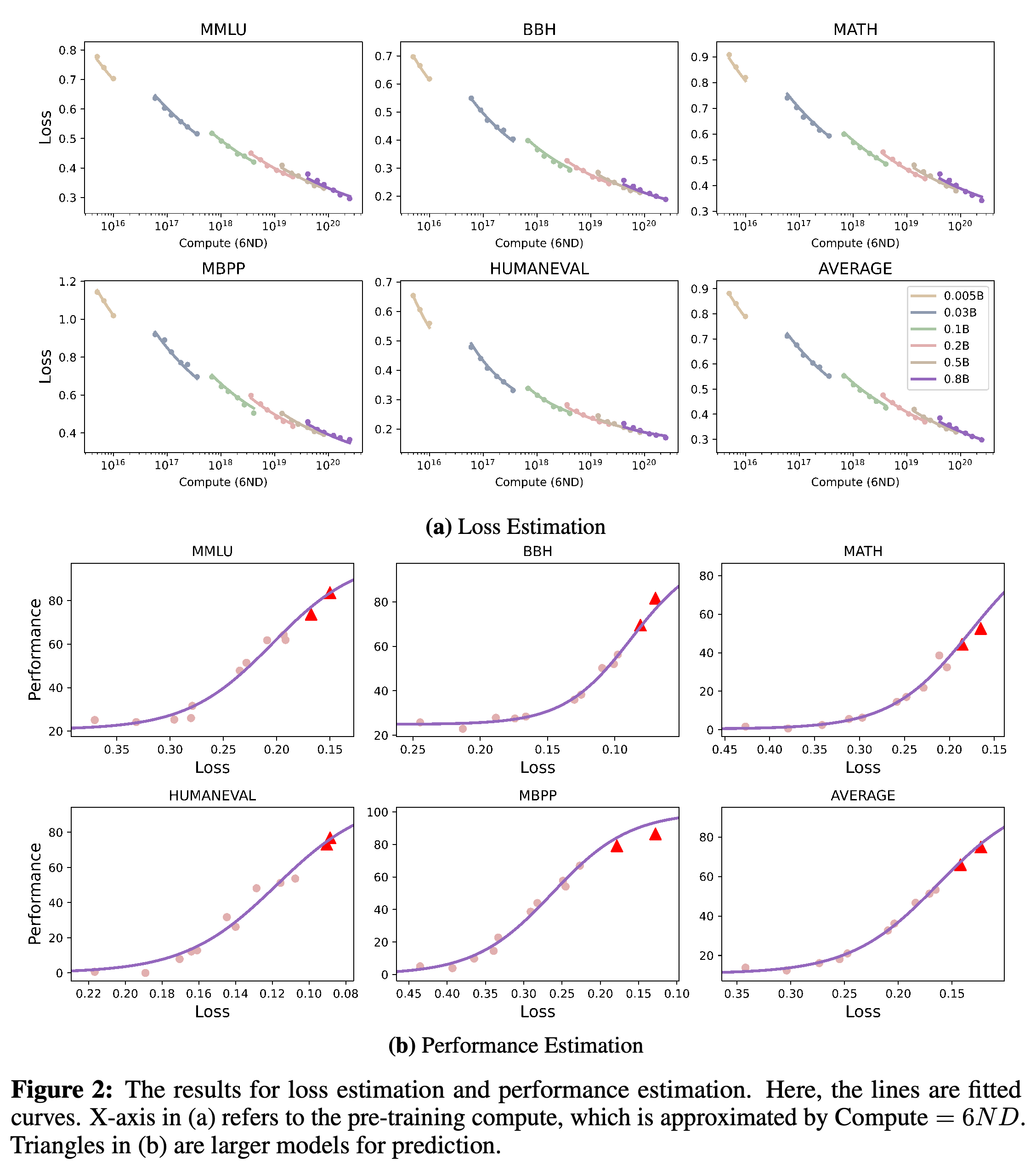
Figure 2 shows decreasing conditional loss with increasing pretraining computation and an S-shaped relationship between loss and task performance. To test prediction beyond the fitting range, the authors fit the loss-to-performance curve using models with fewer than 4 billion parameters and reserve two models with tens of billions of parameters for prediction.

The held-out points broadly follow the fitted curves, providing a graphical check within the evaluated model family. This section reports no numerical prediction errors or uncertainty intervals.
Although the prose refers to three downstream tasks, Figure 2 displays all five selected benchmarks and their average.

Conditional-loss scaling and fitted loss-to-performance relationships for five benchmarks and their average, including larger models held out for prediction.

3.3 Densing Law

Densing Law fits the upper envelope of observed model densities using $\ln(\rho_{\max})=A\cdot t+B$, where t is days since Llama-1’s release. The main text reports A ≈ 0.0073, ln(2)/A ≈ 95 days, and R² = 0.912. Highlights instead reports approximately 3.3 months and R² ≈ 0.93.

The authors report Llama-1 densities below 0.1 and describe recent models such as Gemma-2-9B and MiniCPM-3-4B as reaching approximately 3, although Figure 1 places Gemma-2-9B below that level. They associate density growth with larger and better-cleaned training datasets, citing 1.4 trillion tokens for Llama-1 and 15 trillion for Llama-3.
Llama-3.1-405B illustrates that high absolute benchmark performance does not guarantee the highest density. The fitted law describes maximum observed density across releases rather than the trajectory of every model.

3.4 Corollaries of Densing Law

Corollaries of Densing Law develops five implications, with observational comparisons for several of them. These include historical application programming interface (API) prices, an MMLU-only comparison across ChatGPT’s release, and densities of compressed models relative to their larger source models.

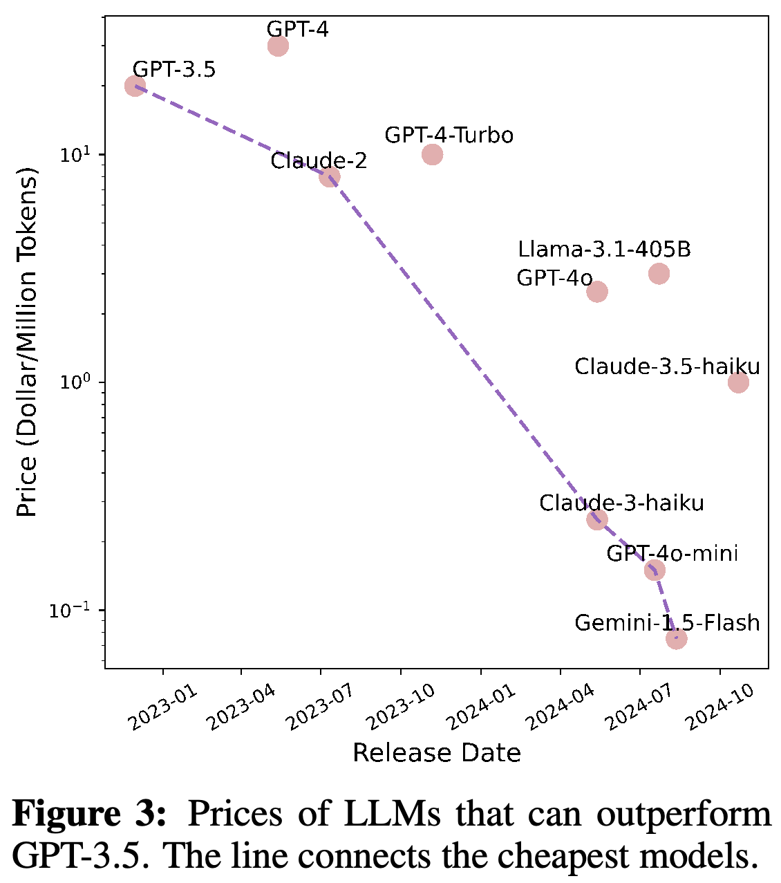
Inference Costs Decrease Exponentially: the paper compares GPT-3.5 at $20 per million tokens in December 2022 with Gemini-1.5-Flash at $0.075 in August 2024, reporting a 266.7-fold reduction and approximately 2.6 months per halving. It attributes price declines to both smaller models and improved inference infrastructure.
Densing Law Meets Moore’s Law: Moore’s Law concerns increasing chip component density. Combining model-density growth with a cited doubling of same-price chip computation every 2.1 years yields the authors’ estimated 88-day doubling of maximum effective model size; this is a derived implication rather than a deployment experiment.
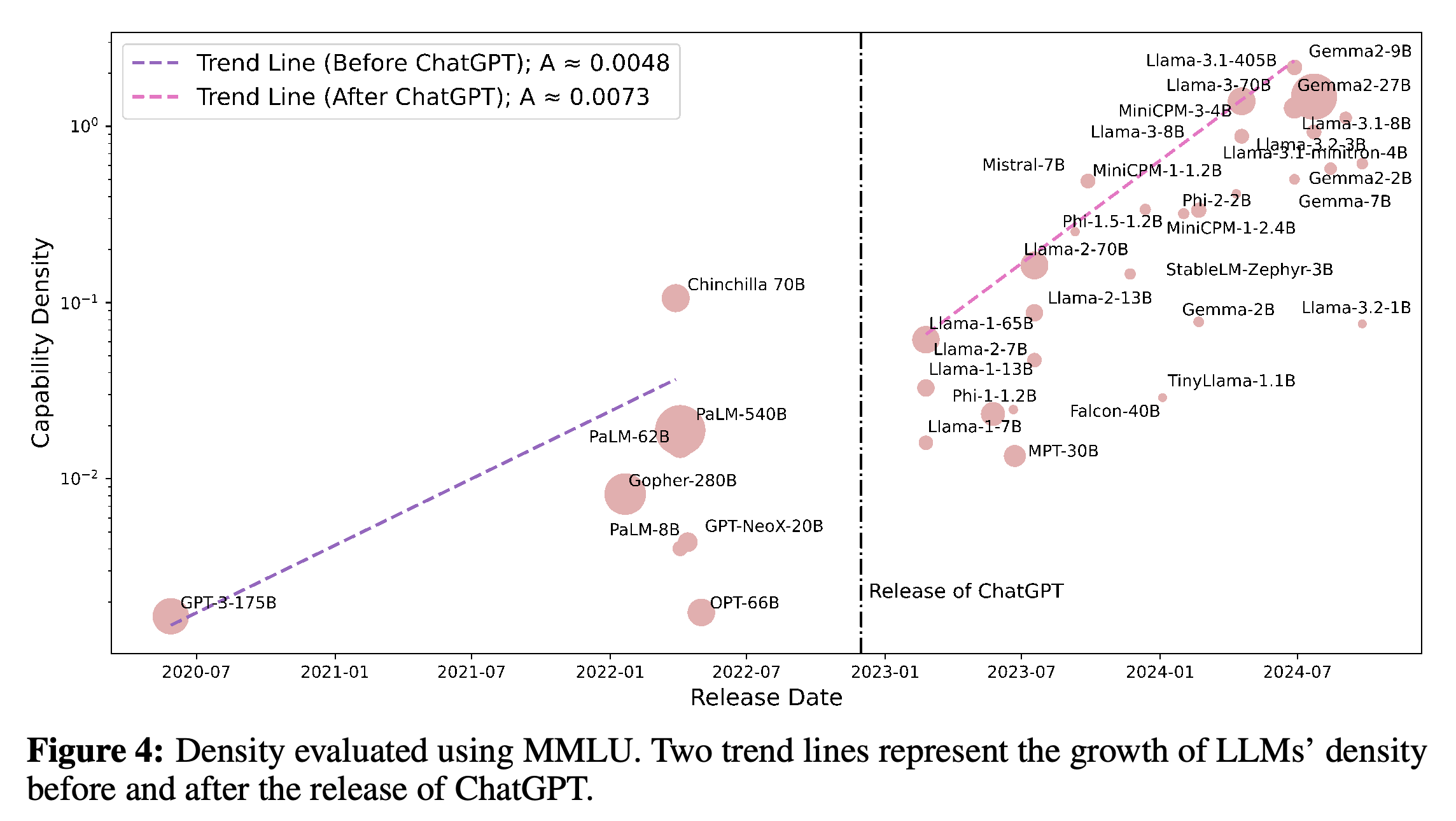
Density Growth Accelerated after ChatGPT’s Release: MMLU-based trend slopes increase from A ≈ 0.0048 before ChatGPT to A ≈ 0.0073 afterward, described as approximately 50% faster growth. Investment and open-source availability are proposed explanations; the comparison does not establish causation.
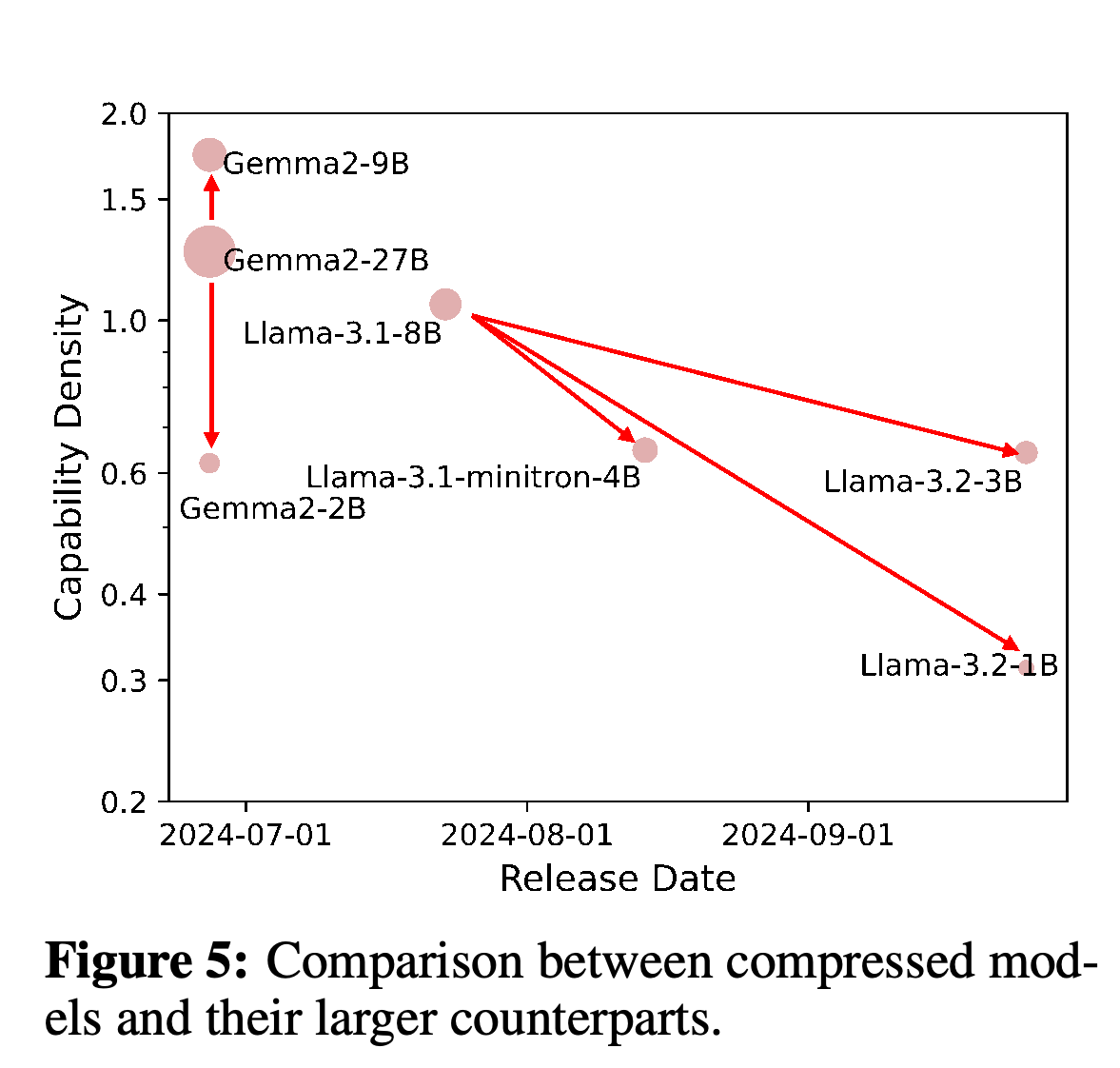
Efficient Compression ≠ Density Improvement: among the plotted compressed models, only Gemma-2-9B exceeds its larger source model’s density. Gemma-2-2B, Llama-3.1-minitron-4B, and Llama-3.2-3B/1B have lower density than their respective source models; insufficient compression-stage training is suggested as a possible explanation.
Towards Density-Optimal Training - Green Scaling Law: the authors advocate improving performance per parameter while considering training expense and short model lifecycles. The paper does not implement or evaluate a new density-optimal training algorithm.

Prices in dollars per million tokens for models described as outperforming GPT-3.5, with a line connecting the cheapest offerings over time.

MMLU-based capability densities with separate growth trends before and after ChatGPT’s release.

Capability-density comparisons between selected compressed models and their larger source models.

4 Discussion

Discussion emphasizes that density is relative to the chosen reference and benchmark suite because model capability cannot be measured comprehensively. It distinguishes scaling relationships within a training setup from Densing Law’s historical trend across successive model releases.

Under sufficient training data, the authors discuss loss scaling as L = AN^(−α) and suggest that improvements in data, algorithms, and architecture could increase α. The historical analysis does not estimate changes in α or isolate the contribution of each factor.
Continued exponential growth is presented as the authors’ expectation based on ongoing investment; its duration is not established. Their further suggestion that models conducting autonomous research could accelerate density growth is speculative.
The discussion calls for updating evaluation datasets as existing benchmarks become less discriminating.

5 Limitations and Future Directions

Limitations and Future Directions identifies benchmark coverage and fairness as central weaknesses: narrow task suites miss evolving capabilities, while contamination and benchmark-directed optimization can inflate scores. The authors propose newly constructed evaluation datasets, extension to multimodal models that process multiple types of data, and a density measure based on inference computation.

The proposed Inference Densing Law would compare effective inference FLOPs with actual inference FLOPs, where FLOPs count floating-point operations. This would account for additional reasoning computation that parameter count alone does not capture.
Multimodal density and inference-computation density remain future directions. The reported empirical law concerns language-model base checkpoints under the selected prompting conditions.

6 Conclusion

The conclusion restates capability density as a method for comparing training quality across model sizes and summarizes an approximately three-month doubling trend among open-source base models released since 2023. Matching present performance with half as many parameters is an extrapolation of that empirical frontier under the selected reference and benchmark conditions.

Appendix

The supplied 16-page PDF contains no appendix; pages 13–16 contain References.

Brief Thoughts

Expressing task performance as an equivalent reference-model size gives the metric a clearer comparison basis than dividing raw accuracy by parameter count. Figure 2 provides a limited check beyond the estimator’s fitting range, but the paper supplies no uncertainty analysis for the frontier growth rate, and its headline and main-text fit statistics differ. The approximately three-month doubling time is a historical result for this evaluation setup. Reference choice, contaminated scores, and changing benchmark coverage can alter density estimates. The API-price comparison and compression examples support observations about the selected models. General claims about deployment cost or compression effectiveness require additional measurements of hardware, serving implementation, and inference length.