Neural Approximation of Graph Topological Features | Summary

This article explains the key points of Neural Approximation of Graph Topological Features.

• 2022-01-28 (arXiv), 36th Conference on Neural Information Processing Systems (NeurIPS 2022)
• Yan, Zuoyu, Ma, Tengfei, Gao, Liangcai, Tang, Zhi, Wang, Yusu, Chen, Chao.
• Wangxuan Institute of Computer Technology, Peking University, IBM T. J. Watson Research Center, Halıcıoğlu Data Science Institute, University of California, Department of Biomedical Informatics, Stony Brook University
• Paper (Reviewed version: v4 (2022-11-15))

Read this article in Korean

Summary

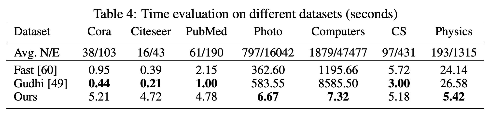
• Computing graph summaries that capture connected components and loops can bottleneck graph learning on large, dense graphs. On 1,000 two-hop neighborhoods from Computers, the proposed neural approximation took 7.32 seconds versus 1195.66 seconds for the Fast exact algorithm, while downstream scores using predicted summaries were comparable to scores using exact summaries.
• The method predicts extended persistence diagrams (EPDs), point sets recording when graph structures appear and disappear as a threshold changes. It reformulates their computation as edge-wise prediction and trains a graph neural network to imitate parts of Union-Find, an algorithm for maintaining connected components.
• Across five neighborhood-graph datasets, the proposed Persistence Diagram Graph Neural Network (PDGNN) reported lower approximation errors than the tested baselines. Exact algorithms were faster on small Cora and Citeseer neighborhoods, and some unusual diagrams remained difficult to approximate.

1 Introduction

Persistent homology summarizes graph topology across thresholds, but computing EPDs for many local neighborhoods can dominate a learning pipeline. The challenges include matrix reduction and supervision of a variable-size point set using a matching-based distance.

2 Background: Extended Persistent Homology

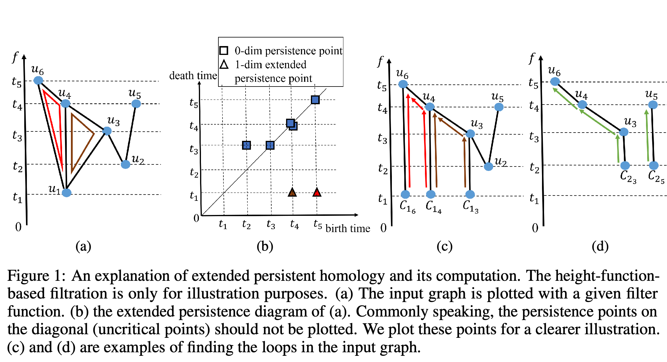
A filter function assigns scalar values to graph elements, and a filtration adds or removes elements in threshold order. A persistence diagram records each feature’s birth and death values; extended persistence also captures independent loops that ordinary persistence leaves without a finite death.

• The paper approximates the union of the ordinary 0D diagram for connected components and the 1D extended diagram for loops; the global minimum and maximum are obtained separately.

The example links connected-component and loop events in a filtered graph to points in its diagram; the split-component examples illustrate how loop pairings are found.

3 Algorithm Revision: Decomposing EPD into Edge-Wise Paring Predictions

Each diagram point corresponds to a vertex-edge or edge-edge pairing, so the computation can be expressed as a prediction for each edge. The authors decompose the exact calculation into Union-Find subroutines and prove in Theorem 3.1 that Algorithm 2 produces the same 1D EPD as the standard algorithm.

• For each vertex, upper-edge splitting places its higher-valued incident edges in separate components; subsequent mergers identify loop persistence points.

4 A Graph Neural Network for EPD Approximation

The framework combines edge-wise prediction with PDGNN, a backbone whose aggregation and message passing are designed around the decomposed Union-Find computation.

4.1 EPD computation as a edge-wise prediction problem

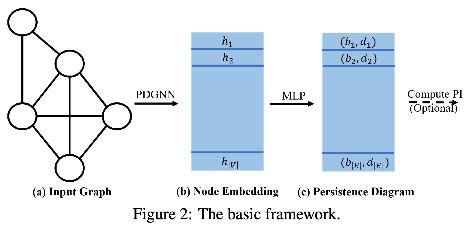
PDGNN embeds nodes initialized with their filter values, and a multilayer perceptron maps concatenated endpoint embeddings for each edge to a two-coordinate persistence point. The implementation uses bounded-size node features, approximating the parallel subroutines without features proportional to graph size.

Node embeddings are produced from the input graph, then an edge-level prediction produces persistence points that can optionally be converted to a persistence image.

4.2 PDGNN

PDGNN concatenates sum and minimum aggregation to model component root finding, and uses endpoint features and attention-derived edge weights in messages to model edge operations. Training uses a 2-Wasserstein distance, a matching-based distance between predicted and ground-truth diagram points, with the matching constraint described in the appendix.

5 Experiments

Experiments use citation, Amazon shopping, and coauthor graphs, extracting one- or two-hop neighborhoods and four filters: distance based on Ollivier-Ricci curvature, a graph metric; heat kernel signatures at temperatures 10 and 0.1; and node degree. The paper evaluates approximation, node classification, link prediction, and computation time; code is listed at https://github.com/pkuyzy/TLC-GNN.

5.1 Approximation Quality

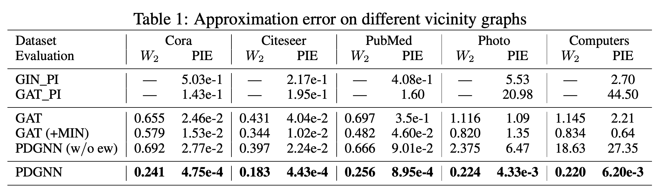
Neighborhoods are randomly split 80%/20% for training and testing; evaluation reports mean 2-Wasserstein distance and persistence image error, the squared error between vectorized diagrams. On Cora, PDGNN achieved 0.241 and 4.75e-4 respectively, compared with 0.579 and 1.53e-2 for GAT (+MIN), a graph attention network with minimum aggregation; removing edge weights also increases error.

PDGNN has the lowest reported Wasserstein and persistence image errors across the five datasets; removing edge weights substantially degrades results, especially on Computers.

5.2 Downstream Tasks

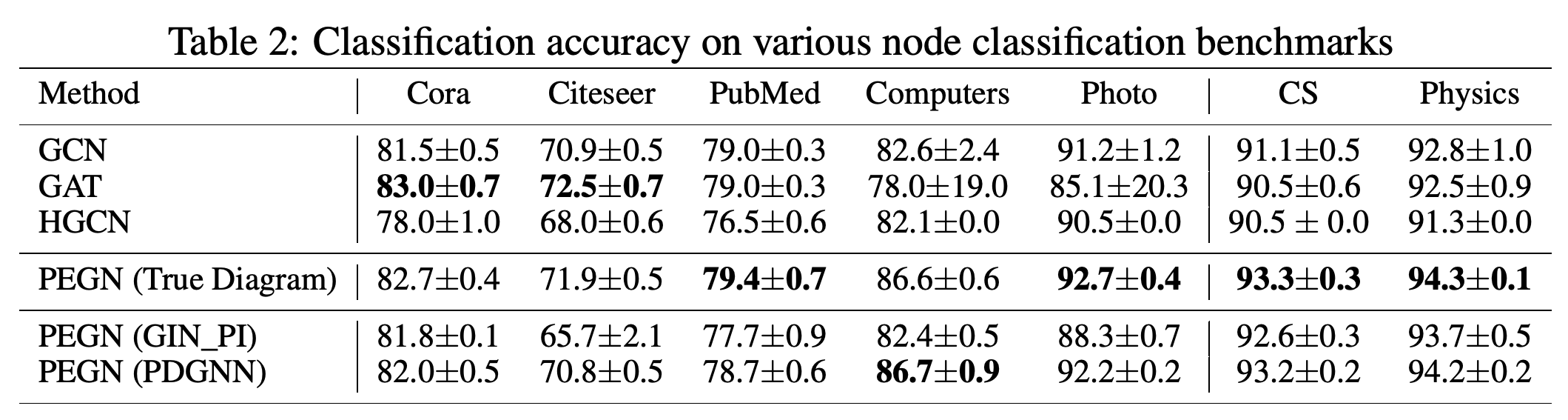
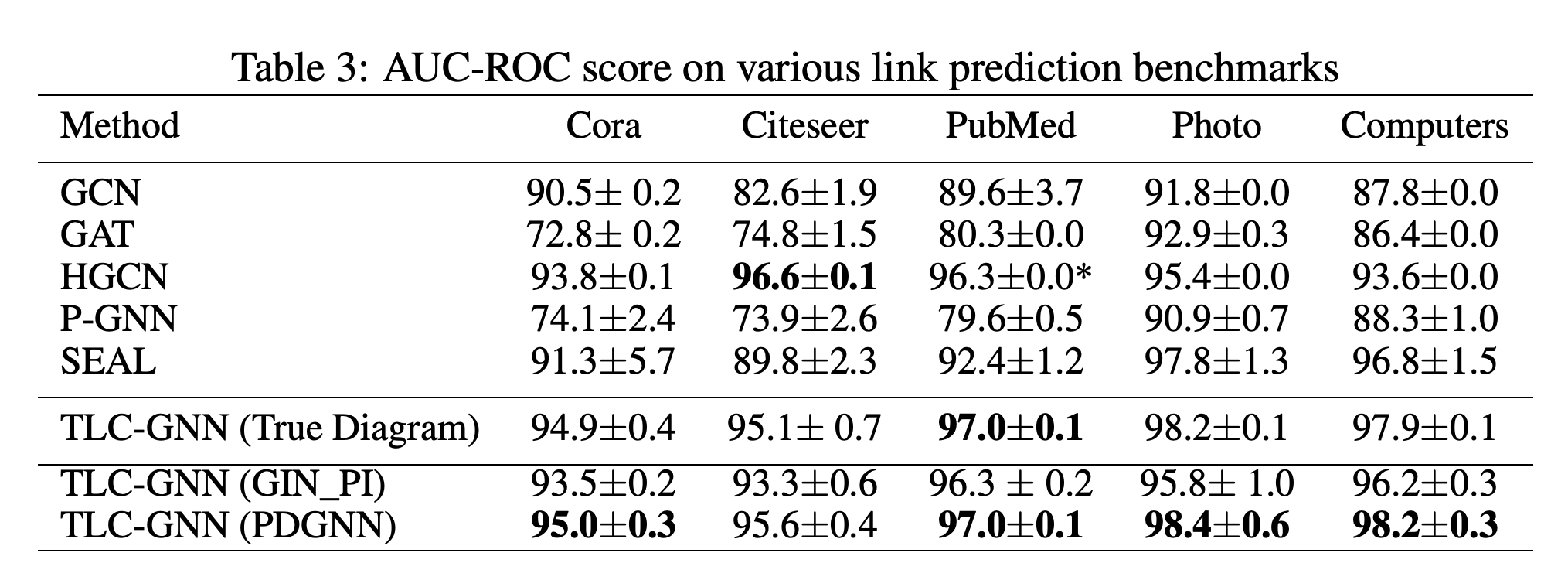
For node classification, training uses 20 nodes per class, with 500 validation and 1,000 test nodes; link prediction splits edges 85/5/10% and samples nonexistent edges as negatives. Across 10 runs, the persistence-enhanced graph neural network PEGN with PDGNN on Computers scored 86.7±0.9 versus 86.6±0.6 with true diagrams, while the persistence-based link predictor TLC-GNN scored 98.2±0.3 versus 97.9±0.1 in area under the receiver operating characteristic curve.

Replacing true diagrams with PDGNN predictions preserves similar node classification accuracy across the seven benchmarks, although the values are not identical.

TLC-GNN using PDGNN predictions achieves scores close to those using true diagrams across five link prediction datasets.

5.3 Algorithm Efficiency

The timing experiment extracts two-hop neighborhoods of the first 1,000 nodes and uses the Ollivier-Ricci-based filter. PDGNN took 6.67 seconds on Photo versus 362.60 for Fast, but 5.21 seconds on Cora versus 0.44 for Gudhi, so the benefit depends on the workload.

The neural method is slower on the smallest neighborhoods but substantially faster on Photo and Computers, which have far more nodes and edges per neighborhood.

6 Conclusion

The authors conclude that algorithm-guided neural approximation retains useful topological information in the tested downstream tasks and reduces computation time on large graphs. Their transfer experiment also tests a model pretrained on Photo against other graph datasets.

Appendix

• The supplement reviews persistent-homology learning, neural algorithm execution, and faster exact computation. It proves correctness of the exact decomposition, gives a sequential Union-Find algorithm for the 0D diagram, and reports O(|V||E|α(|E|)) time for the sequential 1D calculation, where α is the inverse Ackermann function; the proof does not establish exactness of the learned model.
• The datasets include citation networks, Amazon shopping graphs, and coauthor graphs; the supplement states that the benchmark assets are provided under the MIT license. The configuration uses a four-layer graph neural network, a two-layer multilayer perceptron, Adam with learning rate 0.002 and weight decay 0.01, batch size 10, and 20 epochs. During training, predicted points are forced to match ground-truth points rather than the diagonal to avoid collapse; normal matching is used for evaluation.
• With Photo pretraining and one epoch of fine-tuning, PubMed diagram error was 0.360 versus 0.344 under the standard setting. Training-sample experiments show lower diagram error with more samples, while node classification scores remain relatively close; whole-graph experiments omit the Ollivier-Ricci filter because of its cost. An example also shows that directly predicted persistence images can have similar squared error but a different spatial distribution from the ground truth.
• Additional tests cover large sparse graphs and alternative filters; synthetic timing experiments report workload-specific crossover points near 100 nodes and 820 or 766 edges. The authors note that rare diagram distributions can be poorly approximated and topology alone may omit useful semantic information. The checklist says training details and error bars are provided and states that code would be released upon acceptance; the main text separately supplies a code URL.

Brief Thoughts

The diagram-level ablations and downstream comparisons provide complementary evidence: the full model reduces approximation error while retaining similar task scores to exact diagrams. The timing results should be read alongside the small-graph slowdown and the limited transfer and filter settings tested.