Physical Design using Differentiable Learned Simulators | Summary

This article explains the key points of Physical Design using Differentiable Learned Simulators.

• 2022-02-01 (arXiv)
• Allen, Kelsey R., Lopez-Guevara, Tatiana, Stachenfeld, Kimberly, Sanchez-Gonzalez, Alvaro, Battaglia, Peter, Hamrick, Jessica, Pfaff, Tobias.
• DeepMind, UK
• Paper (Reviewed version: v1 (2022-02-01))

Read this article in Korean

Summary

• The paper addresses inverse design: choosing the shape of a physical object to produce a desired behavior. When designs were evaluated with the reference physical simulators, gradient-based optimization through learned simulators outperformed sampling-based optimization on fluid tasks and produced airfoil drag comparable to a specialized solver.
• The authors train graph neural networks, which represent physical systems as connected nodes, to predict physical states and backpropagate through simulated trajectories to update designs. The same underlying architecture supports up to 625 design parameters and fluid trajectories of up to 300 steps without task-specific simulator fine-tuning.
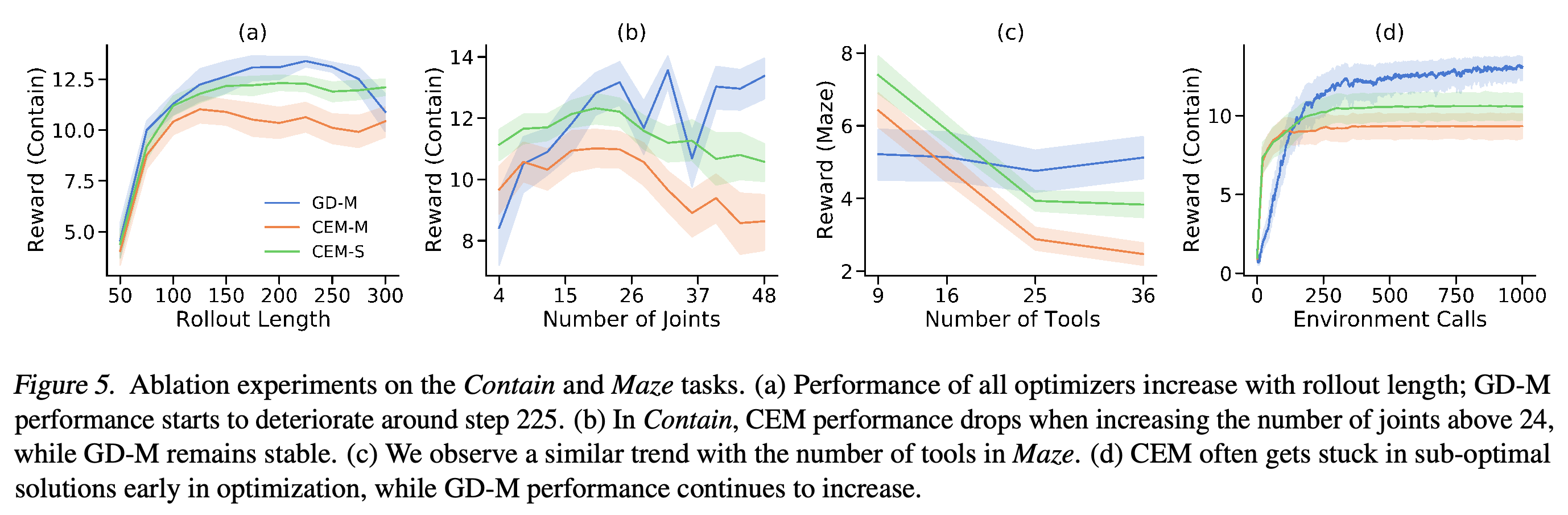
• In one rollout-length experiment, design quality deteriorates beyond roughly 225 steps, and optimization can stall if a tool loses contact with the fluid and its gradient becomes zero. The airfoil timing comparison uses different hardware for the learned model and the specialized solver.

1. Introduction

Classical physical simulators may be slow, specialized, or unable to provide gradients, while learned simulators can accumulate prediction errors and encounter states unlike their training data. The paper tests whether pretrained graph-based simulators are accurate and smooth enough for high-dimensional design optimization over long trajectories.

2. Background

Prior learned generators and scoring functions can accelerate inverse design, but limited generalization may restrict designs to configurations near training examples or require model refinement. The authors instead learn physical dynamics independently of the downstream design objective.

3. Problem Formulation

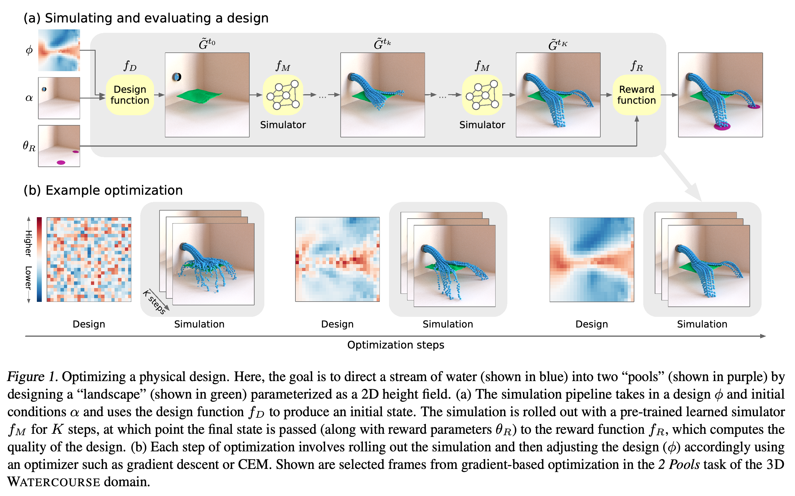
The running example designs a landscape that directs water into two pools. A differentiable design function creates an initial scene, a simulator advances it, a reward function scores the outcome, and an optimizer adjusts the landscape.

The pipeline connects a parameterized landscape to a learned rollout and a final reward; successive designs develop a channel that splits the water stream.

3.1. Learned simulators

MeshGraphNets is a message-passing graph neural network that updates node and edge representations for physical simulation (Pfaff et al., 2021). It represents airfoil meshes with vertices and edges, fluid particles with proximity-based edges, and 3D WATERCOURSE with a hybrid graph; repeated predictions form a rollout, or trajectory of simulated states.

3.2. Optimizing design parameters

Adam updates design parameters by differentiating the learned-model reward through the design function and the full rollout. The cross-entropy method (CEM), a gradient-free optimizer that samples and updates a population of designs, supplies baselines using either the learned simulator (CEM-M) or the reference simulator (CEM-S); gradient descent with the learned simulator is called GD-M.

• Unless otherwise noted, final designs are scored with the reference simulator, including designs found using the learned model.
• CEM uses 20–40 simulator evaluations per optimization step, whereas Adam evaluates one candidate per step. The reference simulators are non-differentiable, so a direct GD-S baseline is unavailable.

4. Design Tasks

The experiments span three domains with different reference simulators, used to generate training data and evaluate designs. The tasks cover fluid-directed tools, water-routing landscapes, and aerodynamic shape optimization.

4.1. 2D FLUID TOOLS

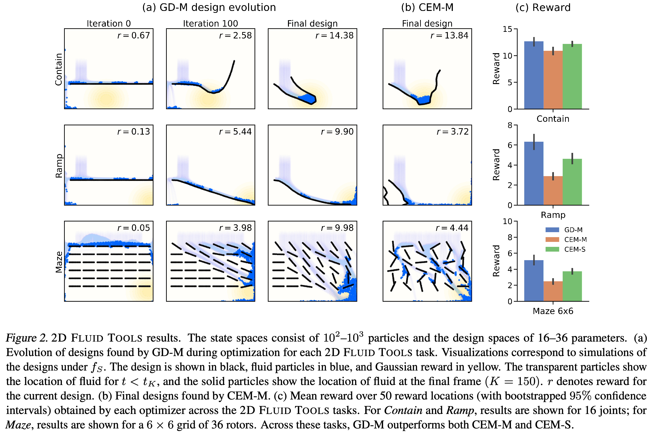
In 2D FLUID TOOLS, Contain and Ramp optimize joint angles of a segmented tool, while Maze optimizes rotations of multiple tools to guide fluid toward a target. Tasks use 4–48 design parameters, 10²–10³ fluid particles, and up to 300 simulation steps; training scenes contain only one to four straight segments (Sanchez-Gonzalez et al., 2020).

4.2. 3D WATERCOURSE

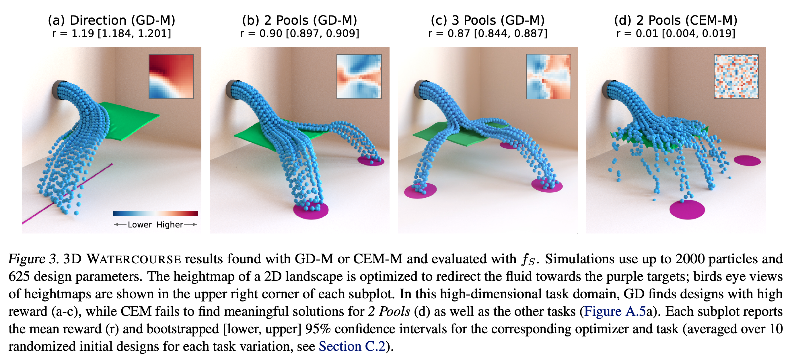
In 3D WATERCOURSE, a 25 × 25 heightmap gives 625 parameters for a landscape beneath a water stream. Direction redirects the stream, while 2 Pools and 3 Pools split it toward targets; simulations run for 50 steps and the main text reports up to 2048 particles.

4.3. AIRFOIL

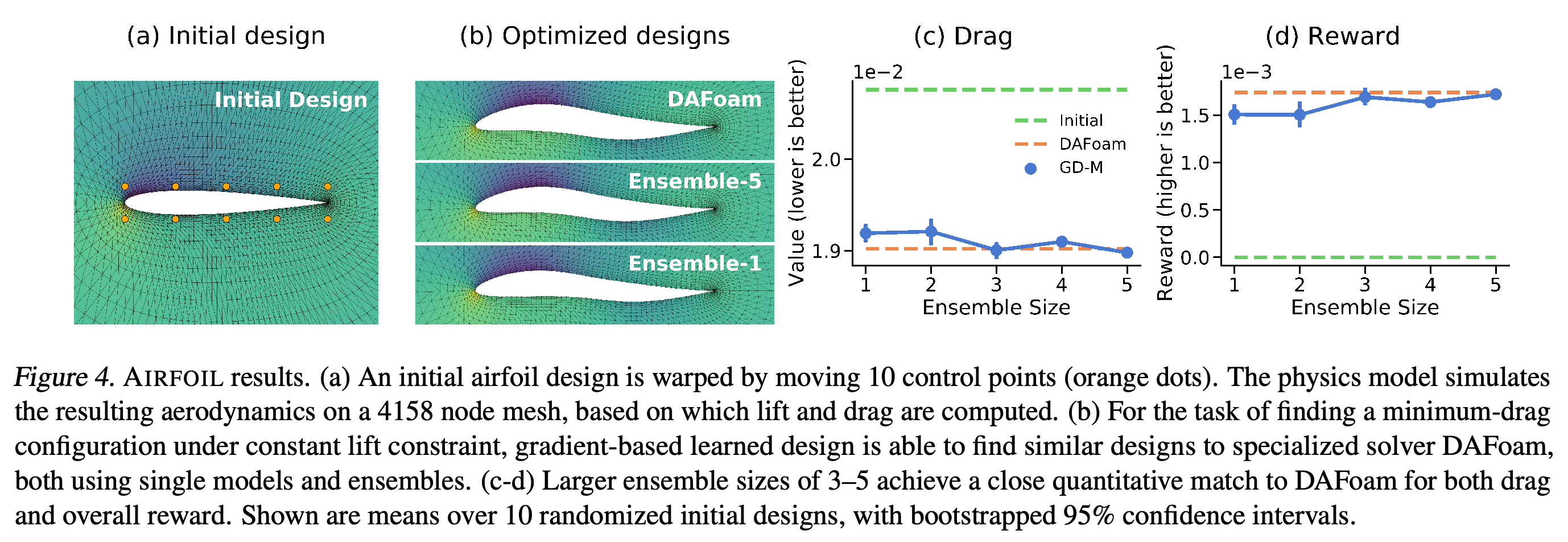
AIRFOIL minimizes the drag of a two-dimensional wing profile while constraining lift and shape. Ten control points deform the profile, and the OpenFOAM fluid solver evaluates airflow on a 4158-node mesh.

4.4. Model learning and optimization

Each domain uses the same underlying graph-network architecture, with identical hyperparameters for the two fluid domains and minor changes for the steady-state airfoil task. Models are trained for next-step prediction on task-independent data and used for design optimization without further fine-tuning.

5. Results

The authors evaluate optimized designs with the reference simulators and provide examples at https://sites.google.com/view/optimizing-designs. The experiments examine overall performance, rollout stability, generalization, ensembles, scaling, and optimization cost.

5.1. Overall results

Across the illustrated 2D FLUID TOOLS tasks, GD-M improves mean reward by 16.1–118.9% over CEM-M and 3.9–37.5% over CEM-S. In 3D WATERCOURSE, CEM-M performs 30–85× worse; in AIRFOIL, GD-M obtains drag coefficients of 0.01898–0.01919 across ensemble sizes versus 0.01902 for DAFoam, a specialized aerodynamic solver (He et al., 2020).

Reference simulations show GD-M forming a container, ramp, and funnel. Reward bars summarize 50 target locations and show GD-M ahead of both CEM baselines for the displayed configurations.

The learned-gradient designs create surfaces that redirect or split water, whereas the displayed CEM-M 2 Pools design leaves most water away from its targets. Reported rewards average 10 randomized initial designs per task variation.

The optimized airfoil profiles resemble the DAFoam solution, and ensembles of three to five models bring drag and reward close to its values across 10 randomized initial designs.

5.2. Model stability & gradient quality

In the Contain rollout-length ablation, GD-M design quality rises until approximately 225 steps and then deteriorates. Across the tested lengths it exceeds CEM-M by 18.1% and CEM-S by 4.4% on average; the authors hypothesize that training noise helps stability and gradient smoothness, but do not establish that mechanism.

5.3. Generalization

The fluid model finds effective curved and multi-obstacle designs despite training on scenes with only one to four straight segments. The authors hypothesize that learned local collision rules support this transfer; the reference solver can also produce particles stuck between obstacles, complicating comparisons in Maze.

5.4. Improving accuracy with ensembles

For AIRFOIL, the authors average gradients from an ensemble of models trained on separate data splits. Five models reach a drag coefficient of 0.01898, compared with 0.01919 for one model and 0.01902 for DAFoam; increasing ensemble size is associated with lower drag and higher reward in their regression analysis.

5.5. Scalability to larger design spaces

With 48 joints in Contain, GD-M exceeds CEM-M by 154.9% and CEM-S by 126.5%; for the 36-joint Maze configuration, the reported gains are 207.4% and 133.7%. The sampling baselines degrade as design dimensions grow, while GD-M remains comparatively effective.

The ablations show GD-M reward peaking around 225 rollout steps and retaining performance as the number of joints or tools grows, while CEM performance declines in larger design spaces.

5.6. Model speed and sample efficiency

AIRFOIL optimization takes 21 seconds with one learned model and 62 seconds with five on a single A100 GPU, versus 1021 seconds for DAFoam on an 8-core workstation, even though GD-M uses 10× more optimization steps. The comparison uses different hardware; in 2D FLUID TOOLS, gradient computation costs about 3× a forward evaluation, but CEM uses 20–40 evaluations per step.

6. Discussion

Across three domains and seven tasks, the study demonstrates that pretrained learned simulators can support gradient-based physical design. Gradient descent can fail in regions with zero gradients, and variable-sized or combinatorial design spaces are difficult to optimize with this approach.

Appendix

• A. Optimizer hyperparameters: The authors sweep major optimizer settings and select CEM sample sizes of 20 for 2D FLUID TOOLS and 40 for 3D WATERCOURSE. Adam uses learning rates of 0.005 or 0.01, with gradient clipping at 10 for the 2D tasks; optimization runs for 1000 steps in 2D and 200 steps in 3D and AIRFOIL.
• B. Model architecture and training: The Encode-Process-Decode network has 10 processor blocks and two-layer node and edge multilayer perceptrons of width 128. It is trained with Adam, batch size 2, training noise, and up to 10 million steps; gradient checkpointing recomputes intermediate activations to reduce memory use over long rollouts (Chen et al., 2016).
• C. Task domains: The 2D fluid model trains on 1000 WaterRamps trajectories, and the 3D model on 1000 trajectories with randomized obstacle planes. AIRFOIL uses 10000 randomized meshes, a 0.1 Mach inflow and a 5.1° angle of attack; its steady-state prediction uses a single model step.
• D. Further results: Learned and reference rewards are close in 3D WATERCOURSE, while discrepancies are larger in Maze, where the material point method (MPM) evaluation solver can produce sticky bottlenecks. Changing to absolute joint angles substantially reduces CEM performance but leaves GD-M reward similar; adding tool translation can move the tool out of contact and leave zero gradients. Additional figures show solutions across rollout lengths, design sizes, and random seeds.

Brief Thoughts

Evaluating the methods with reference simulators shows that the benefit of gradient-based search can outweigh learned-model error on these tasks. The evidence remains simulation-based, and solver artifacts in Maze and different hardware in the airfoil timing comparison limit broader interpretations of physical accuracy and speed.