Scaling Image Tokenizers with Grouped Spherical Quantization | Summary

This article explains the key points of Scaling Image Tokenizers with Grouped Spherical Quantization.

• 2024-12-03 (arXiv)
• Wang, Jiangtao, Qin, Zhen, Zhang, Yifan, Hu, Vincent Tao, Ommer, Björn, Briq, Rania, Kesselheim, Stefan.
• Jülich Supercomputing Centre, TapTap, Tsinghua University, CompVis @ LMU Munich, MCML
• Paper
• Github

Read this article in Korean

Summary

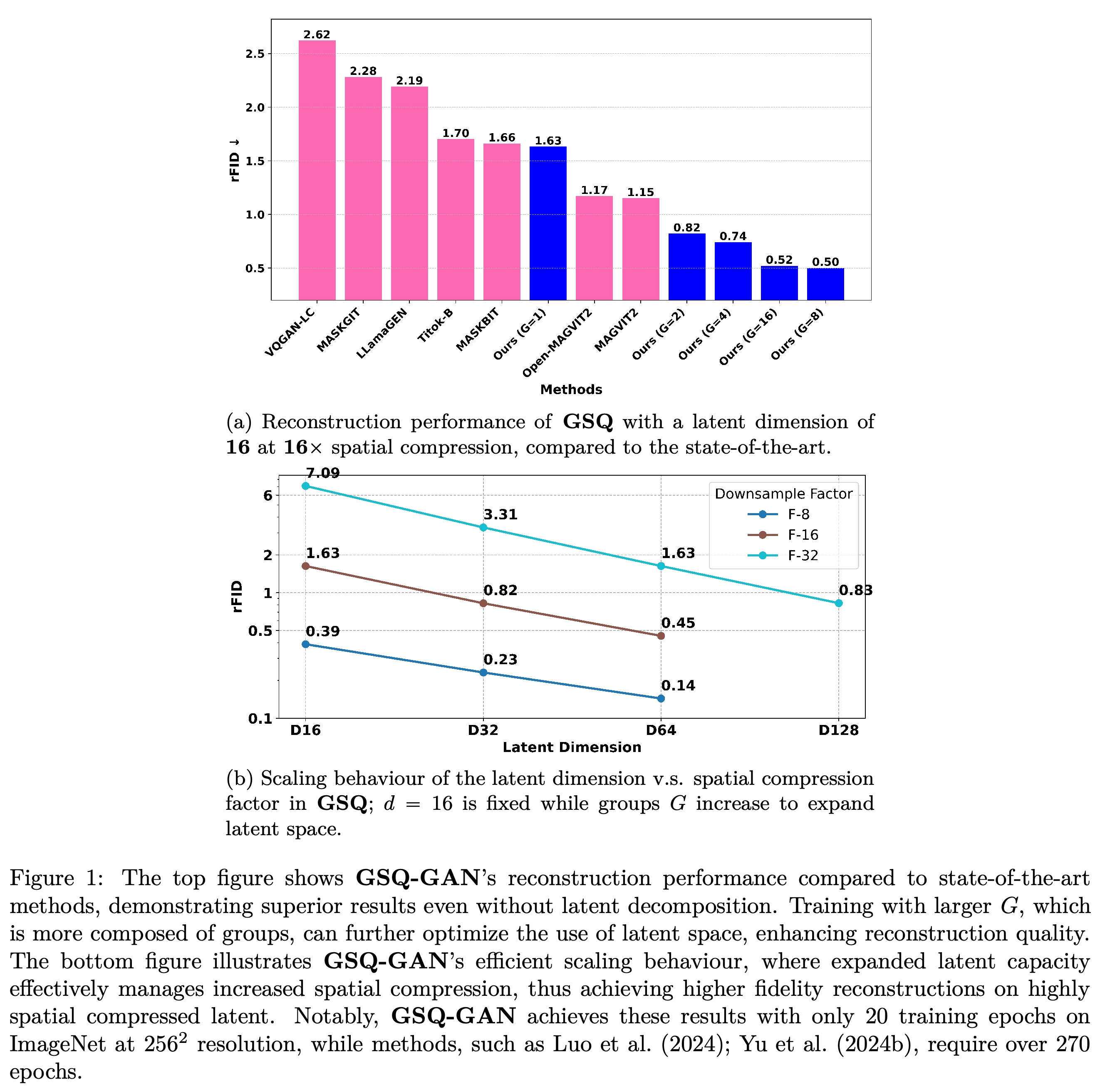
• Image tokenizers, which compress images into discrete representations, must preserve reconstruction quality as their spatial grids become smaller. On ImageNet at 256 × 256 resolution with 16× downsampling along each spatial axis, Grouped Spherical Quantization (GSQ), which quantizes groups of learned image features separately, achieves reconstruction Fréchet Inception Distance (rFID, a distributional reconstruction metric where lower is better) of 0.50 versus the reported 1.15 for MAGVIT2 and 1.17 for Open-MAGVIT2, under different training budgets.
• GSQ combines spherical codebook initialization, which places stored quantization vectors on a unit sphere, normalized lookup, which compares unit-length vectors, and latent decomposition, which splits encoded feature channels into groups. Its tokenizer trained with a generative adversarial network (GAN) objective, GSQ-GAN, uses a discriminator that distinguishes original from reconstructed images; the scaling experiments run for 50,000 steps, or 20 epochs.
• The scaling results depend on spatial compression: without grouping, smaller latent dimensions work better at 8× downsampling, whereas grouping enables larger latent representations to improve reconstruction at 16× and 32× downsampling. The paper evaluates reconstruction and does not test downstream image generation or compare configurations at matched encoded bitrates, the numbers of bits used to represent images.

1 Introduction

The introduction identifies three obstacles to evaluating image tokenizers: inherited GAN hyperparameters can harm reconstruction, legacy vector quantization (VQ), which replaces a vector with a stored codebook entry, can provide weak baselines, and existing scaling studies are incomplete. Finite Scalar Quantization (FSQ), which quantizes individual scalar channels, and Lookup-Free Quantization (LFQ), which uses binary latent components, also couple latent dimension to the number of possible codes.

• The proposed contribution combines an optimized training recipe with independently adjustable group dimension, group count, and codebook vocabulary.
• Figure 1 reports comparisons with prior tokenizers and scaling across 8×, 16×, and 32× spatial downsampling. GSQ uses 20 training epochs, while the caption reports over 270 epochs for the cited MAGVIT2 and Open-MAGVIT2 systems.

The upper panel places the 0.50 grouped result alongside prior 16×-downsampling tokenizers, while the lower panel shows that adding groups at fixed group dimension improves reconstruction across three spatial downsampling factors. The reported 20-epoch budget is shorter than the cited prior training budgets, but the comparison does not hold bitrate or training compute constant.

2 Related Work

The paper places GSQ within compression-oriented image tokenization. Variational autoencoders (VAEs), which encode images into continuous latent representations, precede VQ-VAE, which introduces a discrete codebook; VQ-GAN adds perceptual losses, which compare learned visual features, and adversarial objectives to improve visual reconstruction.

• The reviewed extensions change architectures, quantizers, or losses. Residual Vector Quantization (RVQ) applies successive quantization stages to residual representations.
• A separate research direction transfers semantic representations from pretrained visual models into tokenizers. GSQ concentrates on compression and reconstruction rather than evaluating semantic representation quality.

3 Methodology

The methodology retains an encoder–quantizer–decoder pipeline and changes the quantizer’s geometry and channel organization. It first defines ordinary nearest-code lookup, then introduces grouped lookup to quantize higher-dimensional latent representations in smaller parts.

3.1 Preliminary: VQ Image Tokenizer

The encoder maps an image with height H and width W to an h × w grid of D-dimensional vectors, and the decoder reconstructs the image from its latent representation. The paper defines the spatial downsampling factor as f = H/h = W/w and its latent-to-image element ratio as R = D/(3f²).

• A codebook contains V stored vectors. Ordinary VQ assigns each latent vector to the codebook entry with the smallest squared Euclidean distance.
• R measures latent elements relative to image elements; it does not account for the number of bits needed to encode discrete indices.

3.2 Simple Scaling with GSQ

GSQ divides each D-dimensional latent vector into G groups of d channels, with G × d = D, and quantizes each group separately. Codebook entries are initialized by normalizing samples from a standard Gaussian distribution, and normalized lookup compares unit-length latent and codebook vectors.

• The method uses a shared codebook across groups, allowing group count and group dimension to change independently of its vocabulary size.
• The main text states its normalization exception as G/D ∈ {1, 2}, whereas Appendix C explicitly omits normalization for d = 1 because normalized scalar values collapse to two possibilities. Appendix E also omits lookup normalization for its ungrouped GAN configuration, so the general method description alone does not specify every experimental setting.

4.1 Optimized Training for GSQ-VAE

The initial non-adversarial tokenizer experiments use ImageNet at 128 × 128 resolution, f = 8, V = 8,192, D = 8, and G = 1. Models train for 100,000 steps, or 20 epochs, with batch size 256, learning rate 1 × 10⁻⁴, and an exponential moving average of parameters, which smooths successive parameter updates, with decay 0.999.

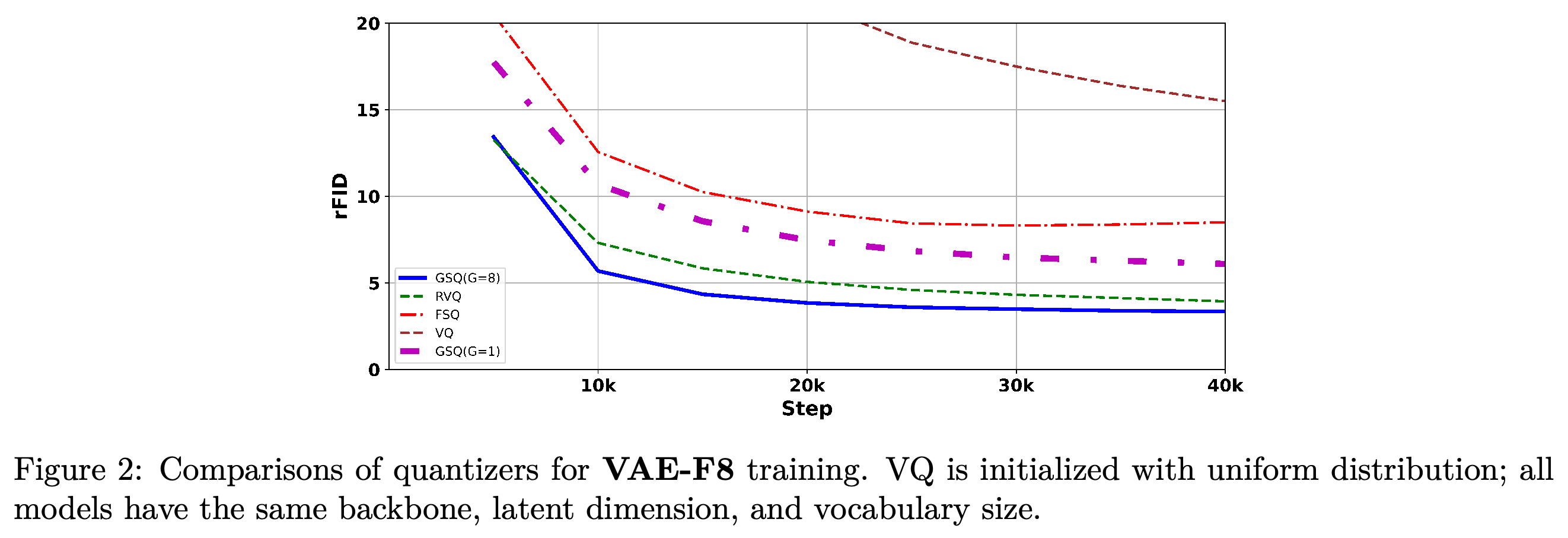
• LPIPS, a learned perceptual image similarity loss, has weight 1.0. The experiments separately examine initialization, lookup normalization, auxiliary losses, architecture, perceptual objectives, and optimizer settings; Figure 2 additionally evaluates G = 8.

4.1.1 Effectiveness of Spherical Quantization

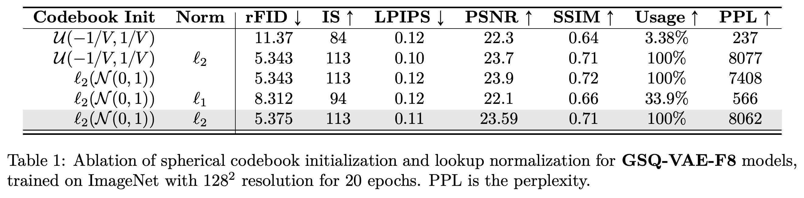
Table 1 shows that uniform initialization without lookup normalization gives rFID 11.37 and 3.38% codebook usage, the fraction of entries selected. Spherical initialization with normalized lookup gives rFID 5.375 and 100% usage, although uniform initialization with normalized lookup also reaches 100% usage and a slightly lower rFID of 5.343.

• Figure 2 holds backbone, latent dimension, and reported vocabulary size constant: GSQ with G = 1 improves over FSQ, and GSQ with G = 8 improves over RVQ on the plotted training curves.
• Table 2 shows a small rFID improvement from entropy loss, an auxiliary objective intended to encourage code utilization, at weight 0.01: 5.375 to 5.281. Larger weights reduce usage, and the tested matrix-information auxiliary loss worsens reconstruction; the authors omit these additional objectives.

Normalization raises uniformly initialized codebook usage from 3.38% to 100%, demonstrating that the poor baseline is strongly affected by lookup geometry. Spherical initialization with normalized lookup also achieves full usage, although its rFID of 5.375 is slightly worse than the 5.343 of normalized uniform initialization.

With backbone, latent dimension, and reported vocabulary size held constant, the curves favor GSQ over the plotted alternatives. The G = 8 curve improves further over G = 1, although this comparison also changes the number of grouped assignments.

4.1.2 Ablation of Network Backbone

Adaptive Group Normalization, which conditions decoder normalization on the latent representation, and Depth2Scale, which rearranges channel information into spatial resolution during upsampling, slightly worsen rFID in the non-adversarial experiments. Table 3 reports 5.375 without either module, 5.406 with adaptive normalization, 5.562 with Depth2Scale, and 5.531 with both.

• Peak signal-to-noise ratio (PSNR), a pixel reconstruction metric, improves from 23.59 to 23.94 with both modules, illustrating that pixel accuracy and distributional reconstruction quality can move differently.
• The authors retain adaptive normalization and revisit Depth2Scale under adversarial training.

4.1.3 Ablation of Perceptual Loss Selection

The perceptual-loss study compares LPIPS with losses derived from the output scores of ResNet and VGG-16, convolutional visual networks, and Dino, a visual model pretrained without supervision. Table 4 reports rFID 4.250 for Dino with perceptual weight 0.1 and reconstruction weight 5.0, versus 5.406 for LPIPS with both weights 1.0.

• The tested ResNet configurations perform poorly, with rFID ranging from 9.625 to 204. This supports a finding about those configurations rather than a general rejection of ResNet features.
• LPIPS remains the default because the authors prefer its balance of rFID and pixel error; the lowest rFID alone does not determine their choice.

4.1.4 Hyper-parameters optimization for GSQ-VAE

The selected Adam optimizer configuration uses β = [0.9, 0.99], the coefficients controlling its moving averages, and weight decay 0.05, yielding rFID 5.343 in Table 5. This is the best tested rFID, although performance does not improve monotonically with every increase in β.

• A constant learning rate of 1 × 10⁻⁴ without warm-up, an initial period of increasing learning rate, gives rFID 5.343. Adding 5,000 warm-up steps gives 5.406, while the tested decay schedules produce values from 5.468 to 5.781.
• All configurations in Tables 5 and 6 report 100% codebook usage, so their reconstruction differences are not explained by unused entries alone.

4.2 Optimized Training for GSQ-GAN

The adversarial experiments add a discriminator and adversarial loss to the tokenizer and train on ImageNet at 128 × 128 resolution for up to 80,000 steps. The initial learning rate is 1 × 10⁻⁴ for both tokenizer and discriminator, followed by studies of discriminator choice, loss combinations, optimization, regularization, and architecture.

4.2.1 Ablations of Discriminator and Combinations of Adversarial Loss

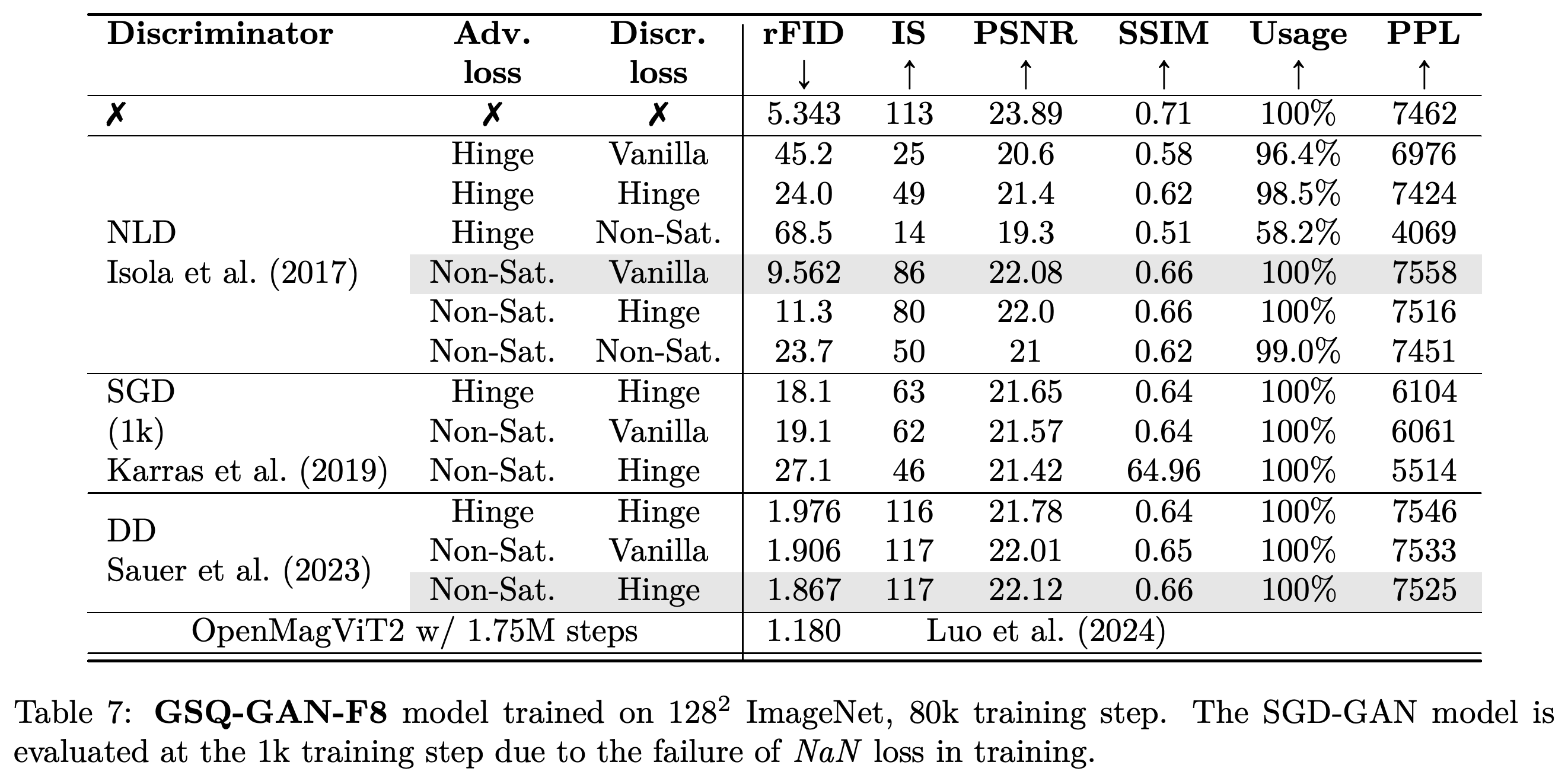
The paper compares an N-Layer Discriminator (NLD), a convolutional discriminator, a StyleGAN Discriminator (SGD), and a Dino Discriminator (DD), which uses pretrained Dino visual features. Loss-pair identifiers list generator then discriminator objectives: V denotes vanilla non-saturating loss, H denotes hinge loss with margin-based discriminator penalties, and N denotes the paper’s improved non-saturating loss.

• Table 7 gives rFID 1.867 for DD-NH, compared with 9.562 for the best initial NLD combination, NLD-NV, and 5.343 without adversarial training. Several NLD loss combinations substantially worsen reconstruction.
• The StyleGAN runs encounter NaN, meaning undefined numerical values, and Table 7 evaluates them at only 1,000 steps. These entries are not completed 80,000-step comparisons.
• Cutout, which masks image regions, combined with color augmentation and translation yields the best 128-resolution result in Table 8. Color and translation alone give the best 256-resolution evaluation result.

DD-NH reaches rFID 1.867, whereas several NLD loss combinations perform substantially worse than the non-adversarial baseline of 5.343. StyleGAN entries are evaluated at 1,000 steps because of numerical failure, so their values do not represent completed runs under the same training duration.

4.2.2 Hyper-parameters Optimization for GSQ-GAN

The adversarial optimizer study selects β = [0.9, 0.99] and adversarial loss weight 0.1. In Table 9, changing β from [0.5, 0.9] to [0.9, 0.99] improves NLD-NV rFID from 9.562 to 3.390, while DD-NH changes only from 1.867 to 1.859.

• Increasing the adversarial weight to 0.5 worsens the tested DD results.
• Table 10 improves rFID from 1.859 with batch size 256 and learning rate 1 × 10⁻⁴ to 1.578 with batch size 512 and learning rate 2 × 10⁻⁴. Batch size 768 does not improve further, showing that the benefit is not monotonic.

4.2.3 GAN Regularization Ablations

Constant adversarial weighting outperforms adaptive weighting in Table 11, and delaying discriminator updates until step 20,000 provides no improvement. Gradient clipping, which limits gradient magnitude, at 2.0 remains the default; reducing NLD weight decay to 1 × 10⁻⁴ slightly improves its rFID, while the same change slightly worsens DD.

• Gradient penalty, a regularizer on discriminator gradients, worsens the tested NLD result. LeCAM, another discriminator regularizer evaluated by the paper, also worsens the listed NLD and DD baselines, despite the main text’s statement that it slightly improves results.
• StyleGAN training remains numerically problematic across the tested remedies. Gradient penalty stabilizes some runs but makes training roughly four times slower, preventing completion within the wall time allocated to 80,000 training steps.

4.2.4 Analysis of Attention Integration

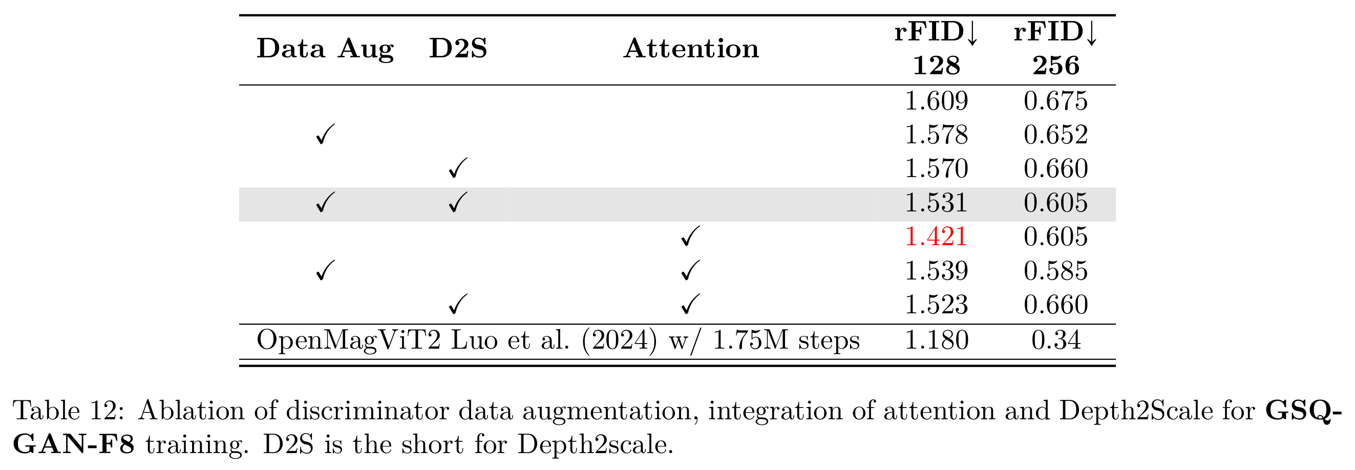
Depth2Scale helps under adversarial training despite its weaker non-adversarial results. Table 12 reports rFID 1.531 at 128 resolution and 0.605 at 256 resolution with data augmentation and Depth2Scale, compared with 1.609 and 0.675 without those additions.

• Attention, which mixes information across latent positions, gives the best listed GSQ 128-resolution result of 1.421 when used alone. Attention with data augmentation gives the best listed GSQ 256-resolution result of 0.585.
• The authors note possible training instability from attention. The table demonstrates cross-resolution inference, but its best GSQ settings differ by evaluation resolution, and the separately reported Open-MAGVIT2 reference has lower rFID at both resolutions after 1.75 million steps.

Depth2Scale and attention can improve adversarial reconstruction, but their effects depend on augmentation and evaluation resolution. Attention alone gives the lowest listed GSQ 128-resolution rFID, while attention with augmentation gives the lowest listed GSQ 256-resolution rFID; the separately reported Open-MAGVIT2 reference remains lower at both resolutions after a longer training run.

4.3 Scaling Behaviors of GSQ-GAN

The scaling experiments train on ImageNet at 256 × 256 resolution for 50,000 steps, or 20 epochs, with batch size 512. This common setup is used to study network capacity, latent dimension, codebook vocabulary, group decomposition, and spatial downsampling.

4.3.1 Network Capacity.

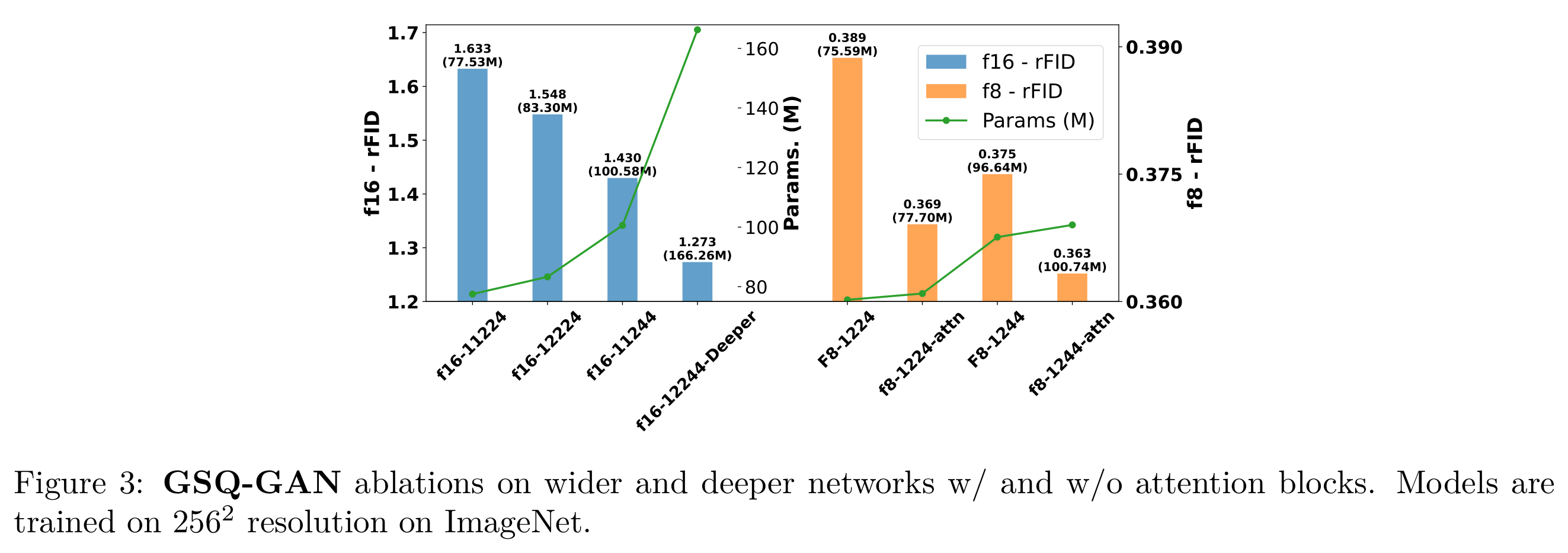
Increasing network width and depth improves reconstruction in the tested configurations. Figure 3 shows the 16×-downsampling models improving from rFID 1.633 at 77.53 million parameters to 1.273 at 166.26 million parameters.

• At 8× downsampling, attention improves the narrower configuration from 0.389 to 0.369 and the wider configuration from 0.375 to 0.363.
• These results establish a quality–capacity tradeoff within the experiment; parameter counts alone do not establish training or inference efficiency.

The 16×-downsampling configurations improve as capacity increases, reaching rFID 1.273 with 166.26 million parameters. The 8× configurations show smaller gains from attention, making the magnitude and parameter cost of improvement visible.

4.3.2 Scaling of Latent Space and Vocabulary.

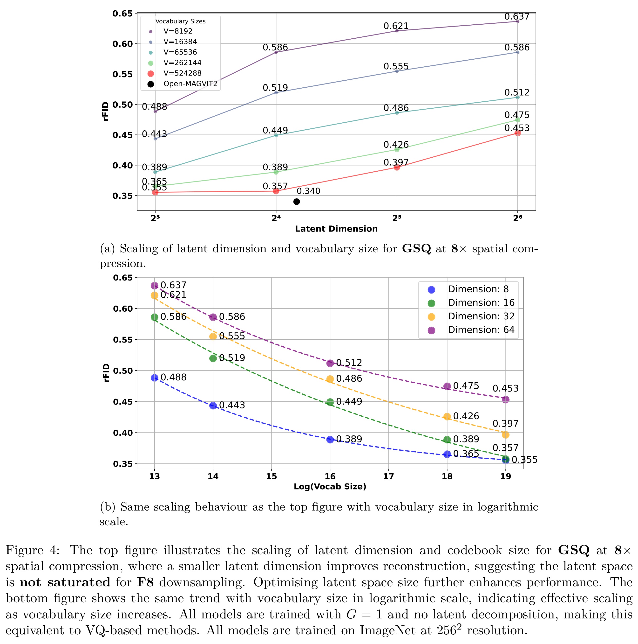
Without grouping, G = 1, the 8×-downsampling study tests latent dimensions 8, 16, 32, and 64 against vocabulary sizes 8,192, 16,384, 65,536, 262,144, and 524,288. Larger vocabularies improve rFID, while smaller latent dimensions perform better throughout this grid.

• For D = 8, increasing vocabulary size from 8,192 to 524,288 improves rFID from 0.488 to 0.355. At vocabulary size 524,288, increasing D to 64 worsens rFID to 0.453.
• Figure 4 includes Open-MAGVIT2 at 0.340, which remains below 0.355. The prose’s claim of outperforming state-of-the-art tokenizers is therefore broader than this particular plotted comparison supports.
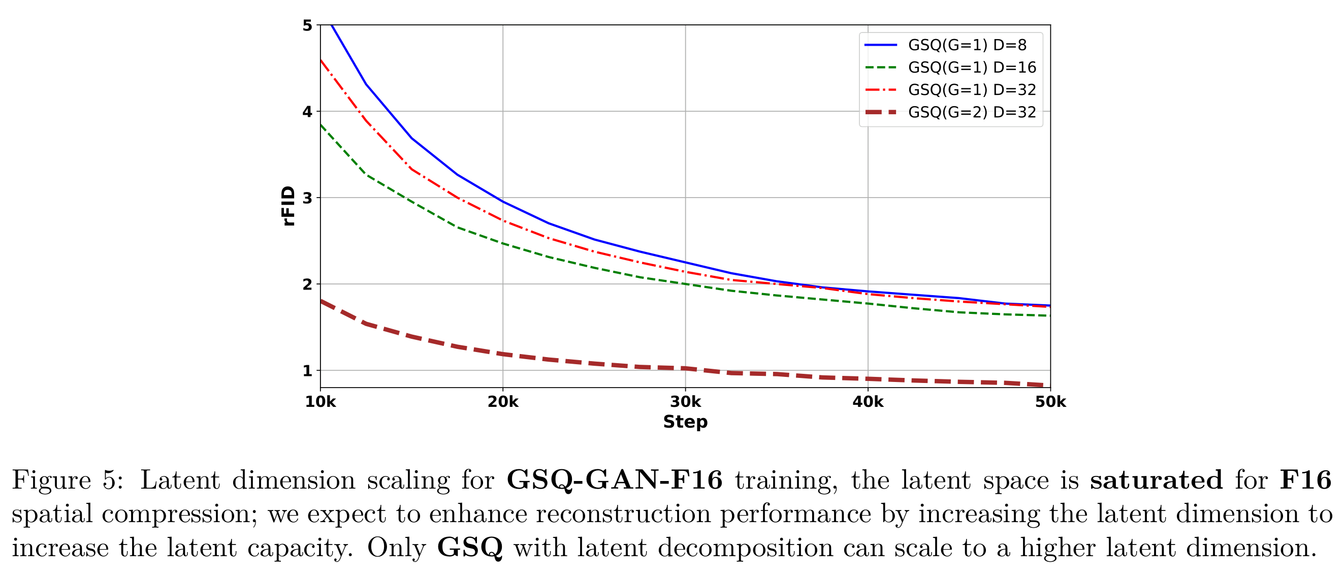
• At 16× downsampling, increasing ungrouped latent dimension beyond D = 16 stops helping; Figure 5 shows that splitting D = 32 into two groups produces a much larger improvement.

Every vocabulary curve favors smaller ungrouped latent dimensions at 8× downsampling, and every dimension benefits from a larger vocabulary. The best plotted GSQ value is 0.355, while the included Open-MAGVIT2 reference is 0.340, qualifying the broader superiority claim in the prose.

4.3.3 Latent Space and Downsample Factor, and Better Scaling with GSQ

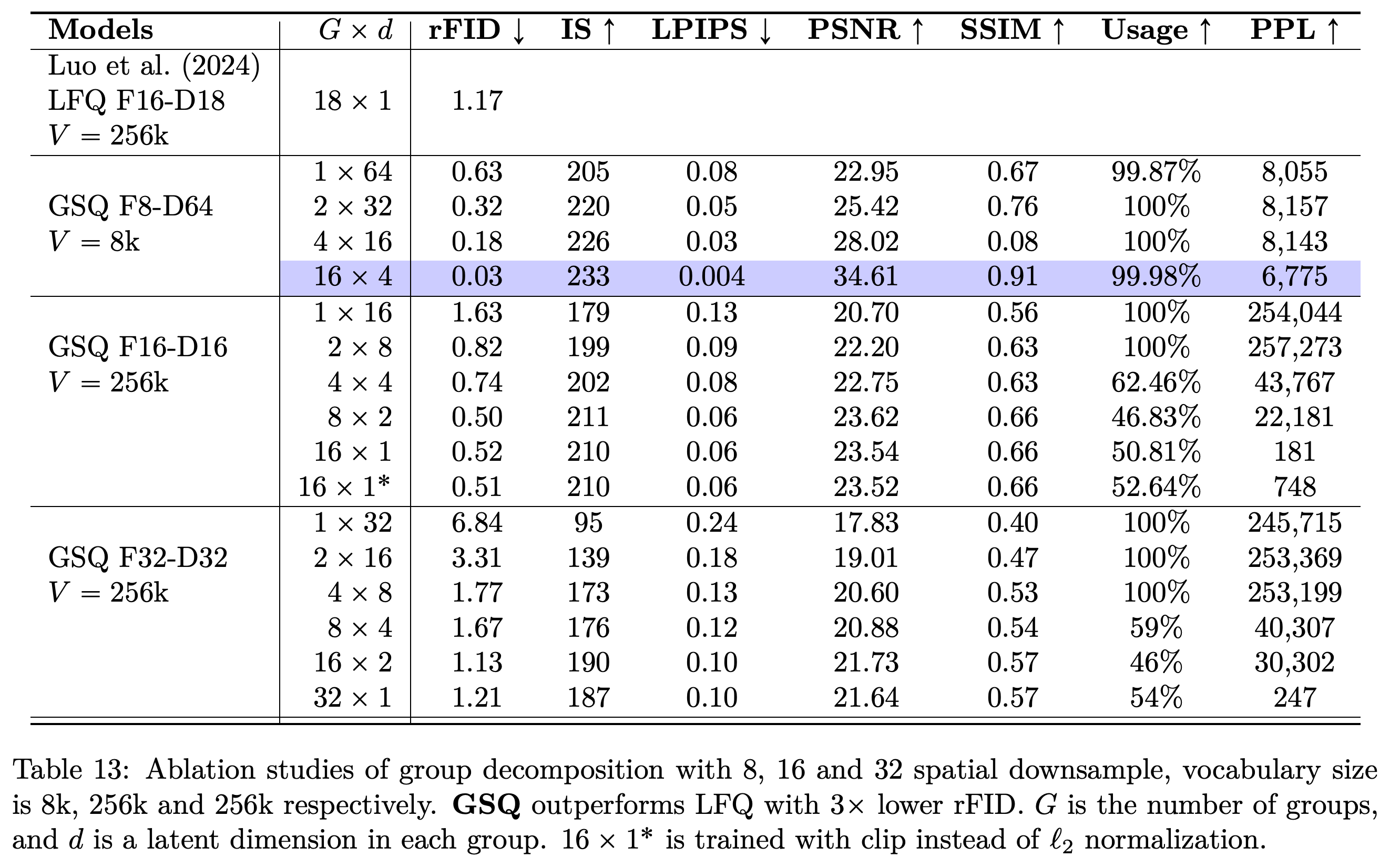
Table 13 tests group decomposition at fixed total latent dimension and per-group codebook vocabulary. For f = 16, D = 16, and V = 256k, increasing G from 1 to 8 improves rFID from 1.63 to 0.50; for f = 32 and D = 32, increasing G from 1 to 16 improves it from 6.84 to 1.13.

• Grouping also changes the number of code indices emitted per spatial position and the effective number of possible combinations. A fixed per-group vocabulary therefore does not imply a fixed encoded bitrate.
• At f = 8, D = 64, V = 8k, and G = 16, rFID reaches 0.03 and PSNR reaches 34.61. The authors describe this as near-lossless reconstruction while acknowledging its limited practical compression value; it is not an exact reconstruction result.
• With group dimension fixed at d = 16, Figure 1b shows that increasing total dimension through additional groups improves reconstruction across f = 8, 16, and 32; at f = 32, rFID falls from 7.09 at D = 16 to 0.83 at D = 128.
• Codebook utilization is not uniformly full: the f = 16, G = 8 configuration reports 46.83% usage, qualifying general statements about 100% utilization.

Increasing an ungrouped latent from D = 16 to D = 32 provides little benefit, whereas dividing D = 32 into two groups markedly lowers the reconstruction curve. This supports grouping under stronger spatial compression, while the extra grouped assignments also change the discrete representation capacity.

At fixed total dimension, grouping substantially improves reconstruction across all three downsampling settings. It also reveals limits to full-utilization claims: the headline F16 configuration with eight groups reaches rFID 0.50 while using 46.83% of its codebook entries.

5 Conclusion

The conclusion attributes GSQ’s reconstruction performance to spherical initialization, lookup normalization, latent grouping, and an optimized training recipe. The experiments support distinct scaling behaviors at low and high spatial downsampling, with grouping particularly useful when larger latent dimensions are needed.

• The demonstrated outcome is improved image reconstruction. Benefits to downstream generative modeling remain a motivation rather than an experimentally established result in this paper.

Appendix

• A Performance of State-of-the-Art Image Tokenizers extends the reconstruction comparison across spatial downsampling settings. Its reported GSQ configuration differs from the headline result, so those entries should not be treated as the same experiment.
• B Networks describes the convolutional encoder and decoder, including resolution and middle blocks, residual connections, optional attention, and adaptive decoder normalization.
• C GSQ and Other Quantizers relates GSQ to existing quantizers through grouping, codebook sharing and normalization. It discusses distance concentration and fits the ungrouped scaling results empirically, without a separate extrapolation assessment; grouped codes also expand the effective representation space.
• D Ablation Studies of VAE documents training, initialization, learning-rate schedules and qualitative reconstructions. Its initialization comparison does not align clearly with the group configuration reported in the main table, leaving that correspondence unresolved.
• E Ablation Studies of GAN provides training, discriminator and loss definitions, including an ungrouped setting without lookup normalization. It records numerical failures and expensive stabilization attempts with the StyleGAN discriminator, alongside qualitative comparisons of discriminator and optimizer choices.
• F Scaling Behaviors documents the scaling-experiment setup and compares qualitative reconstructions as latent dimensions, group counts and spatial downsampling change. These examples supplement the main reconstruction study rather than establishing downstream generation quality.

Brief Thoughts

The clearest evidence comes from the controlled training ablations and fixed-dimension grouping experiments. Table 1 shows how normalization improves a weak conventional baseline, and Table 13 shows additional gains from grouping, supporting the argument that quantizer comparisons depend on both the training recipe and representation structure.

The compression results need to be interpreted alongside the number of emitted indices: additional groups expand the representation, and the paper does not compare encoded bitrate, downstream generator cost, or generation quality. The reported experiments also lack repeated-seed uncertainty estimates, while discrepancies between prose and tables leave some configurations difficult to reproduce precisely.