The Design Space of Tri-Modal Masked Diffusion Models | Summary

This article explains the key points of The Design Space of Tri-Modal Masked Diffusion Models.

• 2026-02-25 (arXiv)
• Bethune, Louis, Turrisi, Victor, Mlodozeniec, Bruno Kacper, Lopez, Pau Rodriguez, Boominathan, Lokesh, Bhendawade, Nikhil, Shidani, Amitis, Pelemans, Joris, Olausson, Theo X., Hjelm, Devon, et al.
• Apple, Google Deepmind, University of Cambridge, MIT
• Paper

Read this article in Korean

Summary

• The Design Space of Tri-Modal Masked Diffusion Models studies pretraining from scratch on text-only, image-text, and audio-text data using one bidirectional transformer and a unified discrete vocabulary. Its main contribution is a controlled investigation of optimization transfer, compute allocation, modality mixtures, masking schedules, and inference settings.
• CompleteP combined with stochastic differential equation (SDE) scaling makes final loss approximately invariant to physical batch size below a critical threshold, separating hardware-oriented batching from optimization behavior. A duration-scaling sweep favors an intermediate drift–horizon allocation, γ* ≈ 0.44, rather than either endpoint used in prior work.
• Across 262 tri-modal models and 24 isoFLOP budgets from 5 × 10^18 to 1 × 10^22, a Kaplan-style scaling law achieves R² = 99.3% and mean relative error of 0.5%. The reported token-optimal frontier is D★(N) = 7754 · N^0.84; despite decreasing optimal tokens per parameter asymptotically, the estimated requirement at 3B scale is approximately 480B tokens, above the approximately 60B Chinchilla reference.
• A pretrain-only 3B model trained on a reported 6.4T tokens produces text, images, and speech, with CC12M FID-Inception 10.06, GenEval overall 48.89, MMLU 41.57, and LibriSpeech-PC FAD 0.368 and WER 0.164. Limitations include weak spatial composition, metric-dependent sampling optima, no observed cross-modal mixture synergies at the tested small scale, and speech evaluation that supplies ground-truth durations.

1 Introduction

The paper motivates masked diffusion as order-agnostic iterative refinement for conditional generation, where evidence can occur at different positions and in different modalities. Joint denoising supports infilling and flexible conditioning without requiring a separate causal factorization for each task.

• The study targets native pretraining rather than initializing from LLaDA or repurposing an autoregressive backbone, making total training-token accounting central to its comparisons.
• The authors acknowledge that naive MDM implementations still have substantial sampling latency relative to autoregressive models; bidirectionality does not itself establish an inference-efficiency advantage.
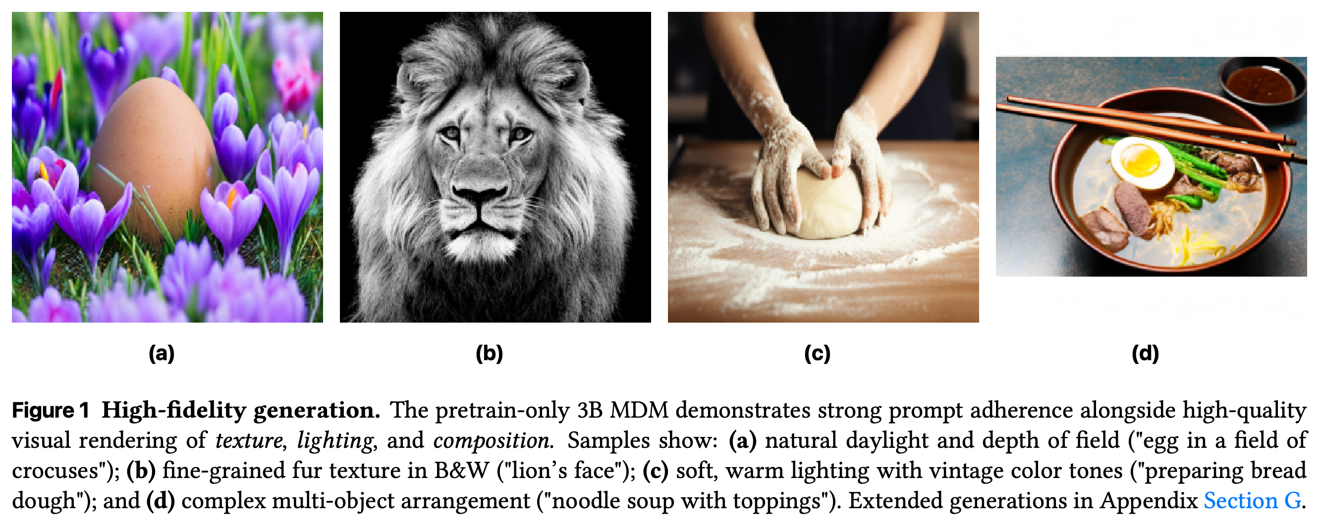
• Figure 1 illustrates selected image-generation capabilities, but qualitative examples do not establish representative prompt adherence or comparative superiority.

The four examples illustrate texture, lighting, and multi-object rendering by the pretrain-only 3B model. They provide qualitative evidence of generation capability, not a measured success rate or comparison against another model.

2 Background and Related Work

The related-work discussion separates masked diffusion for text, image, and audio from unified multimodal models. Generating one modality conditioned on another is distinguished from learning a shared token-level model that can generate multiple modalities.

2.1 Masked Diffusion Models

An MDM progressively replaces discrete tokens with [MASK] and learns the reverse reconstruction process, starting generation from a fully masked sequence. Continuous-time formulations extend the fixed-timestep framework and support training over sampled corruption levels.

• LLaDA and Dream use masked reconstruction objectives associated with a variational likelihood bound, with loss evaluated at masked positions and time-dependent weighting.
• Image tokenizers compress pixels into discrete spatial codes, avoiding the long sequences required by direct categorical pixel modeling.
• For audio, the cited approaches combine discrete diffusion or iterative masking and unmasking with neural audio codecs.

2.2 Multimodal Masked Diffusion Models

Existing unified text–image MDMs include MMaDA, UniDisc, and earlier simultaneous vision-language diffusion models. This work adds audio and jointly pretrains all three modalities from scratch, while recommending that comparisons report both model size and total training tokens.

• The training categories are text-only, image-text, and audio-text; the data description does not introduce directly paired image-audio examples.
• The formulation supports multiple conditioning directions, but the main quantitative results cover language benchmarks, text-to-image generation, and text-to-speech generation.

3 Method

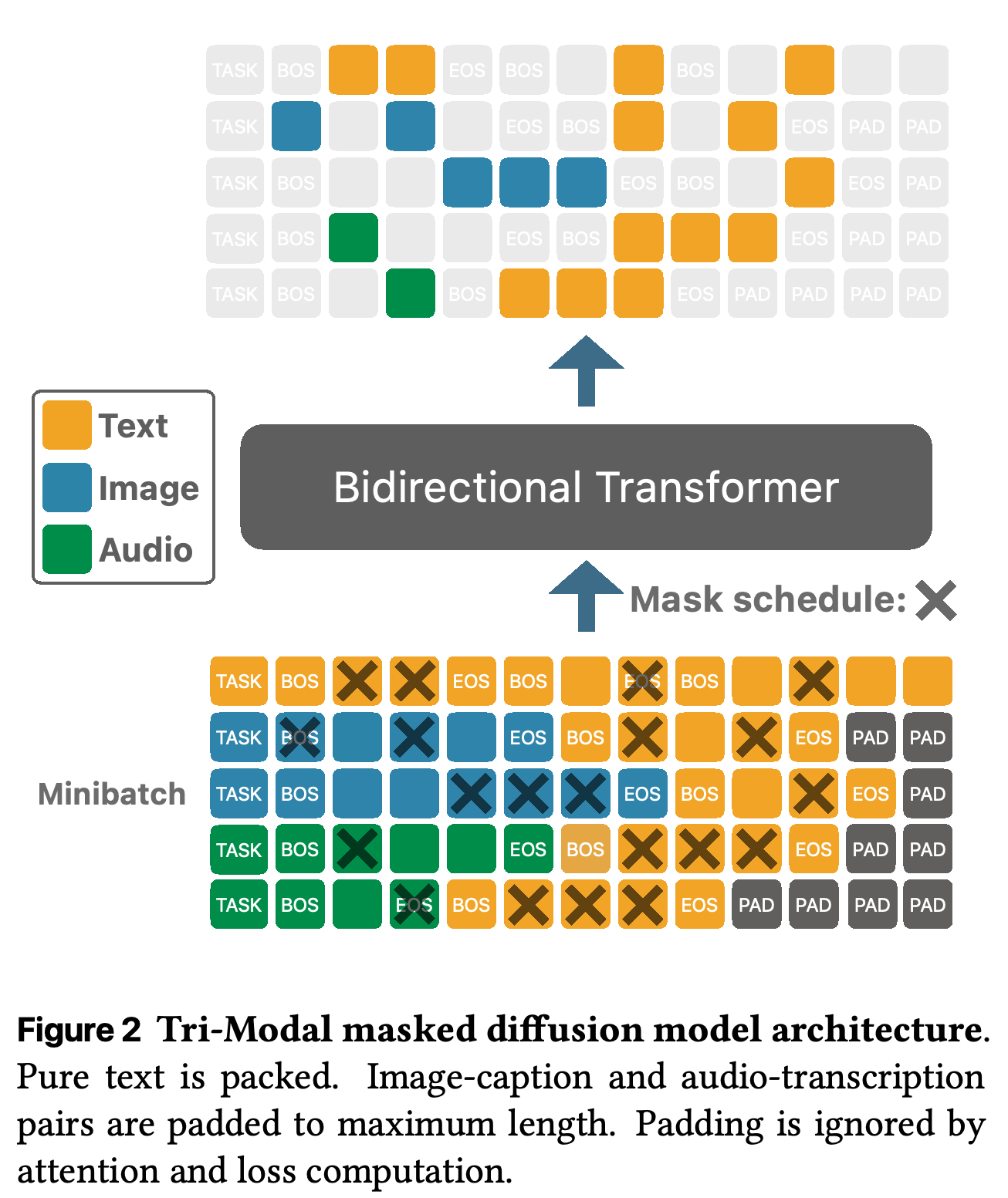
The model combines disjoint text, audio, and image vocabularies with modality-specific BOS, EOS, and MASK tokens, three task tokens, and a padding token. Text sequences are packed and truncated, whereas image-text and audio-text sequences are right-padded after EOStext; task tokens are never masked.

• Independent position-wise masking creates corrupted sequences, and a shared denoiser predicts logits over the unified vocabulary.
• The displayed objective averages reconstruction loss over masked, non-padding positions, applies w(t) = 1/t, and adds a z-loss regularizer. Cut-cross-entropy avoids materializing the full large-vocabulary probability tensor.
• Generation begins with masked target tokens and an observed prompt, then progressively reveals sampled tokens under modality-constrained distributions and a predefined linear unmasking schedule.

One denoiser processes packed text and padded image-text or audio-text sequences. Modality-specific masks retain token-type identity, while padding is excluded from attention and loss.

3.1 Architecture

The backbone is a bidirectional transformer with pre-normalization RMSNorm, SwiGLU MLPs, RoPE, and QK-norm. The 3B model is trained from scratch for 1,000,000 steps with batch size 3072 and sequence length 3256, using SBER-MoVQGAN for images, Higgs Audio v2 for audio, and Tiktoken for text.

• The final configuration has 24 blocks, width 3072, 24 attention heads, and a total vocabulary of 117,698 tokens including special tokens.
• Image training targets 256×256 resolution; audio uses four codec codebooks and a maximum duration of 30 seconds.
• The design shares a transformer backbone and vocabulary-level prediction mechanism rather than adding separate modality-specific generation heads.

4 Hyperparameter Transfer

Hyperparameter transfer replaces infeasible large-scale tuning with a search at a smaller model and token horizon. The study uses CompleteP-based width and depth transfer together with SDE scaling, while examining per-module AdamW tuning as a preliminary extension in Appendix D.

• Global hyperparameter tuning provides the starting point for most controlled ablations.
• Per-module tuning varies learning rate, weight decay, momenta, numerical damping, and initialization across module types and depth groups; the small-scale result does not establish an equivalent gain at 3B scale.

4.1 Eliminating 𝐵opt with SDE Parametrization

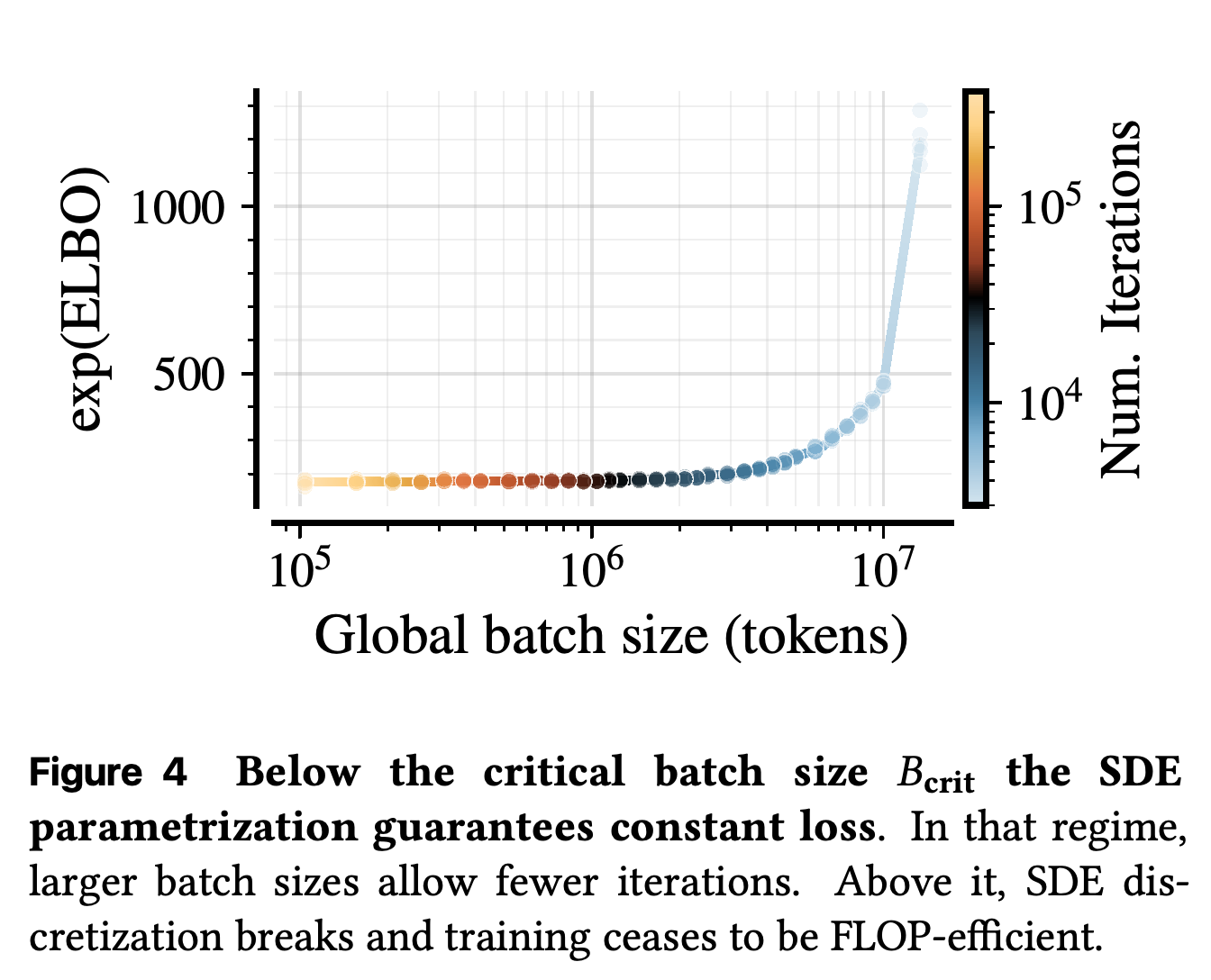
AdamW hyperparameters and batch size jointly determine the continuous optimization dynamics approximated by an SDE. Rescaling the optimizer when physical batch size changes preserves approximately equivalent final loss below Bcrit, removing the need to identify a unique physical Bopt within that regime.

• Figure 4 shows a broad loss plateau followed by degradation at large batches, where too few integration steps undermine the SDE approximation.
• The result requires B ≤ Bcrit, matched token budgets, and the prescribed optimizer rescaling; it does not make arbitrary batch sizes or optimizer settings interchangeable.

Final loss remains nearly flat across a range of physical batch sizes under SDE rescaling, then rises when batching leaves too few optimizer steps. The plateau supports removing physical Bopt tuning within the critical regime.

4.2 Isonoise and Isohorizon Scaling Rules

The duration-transfer rule interpolates between isonoise scaling at γ = 0 and isohorizon scaling at γ = 1 using κ = (Dbase/D)^γ(B/Bbase). AdamW is rescaled as lr = lrbase√κ, β1 = (β1base)^κ, β2 = (β2base)^κ, and ε = εbase/√κ.

• D denotes the training-token horizon in the surrounding experiments, although the explanatory sentence following Equation (4.1) calls it model size.
• The base search uses approximately 3k runs with a 320M-parameter model, including 240M embedding parameters, Dbase = 13B tokens, and Bbase = 256 sequences.
• Changing γ allocates additional tokens between extending the virtual optimization trajectory and reducing gradient-noise fluctuations.

5 Scaling Behavior of MDM under the SDE Transfer Rule

The scaling experiments use CompleteP + SDE transfer, a cosine learning-rate schedule, and 1k steps of linear warmup capped at 25% of total iterations. Width scales with depth while fixing demb/nlayers = 128 to support consistent hyperparameter transfer.

5.1 Scaling Rules for Critical Batch Size

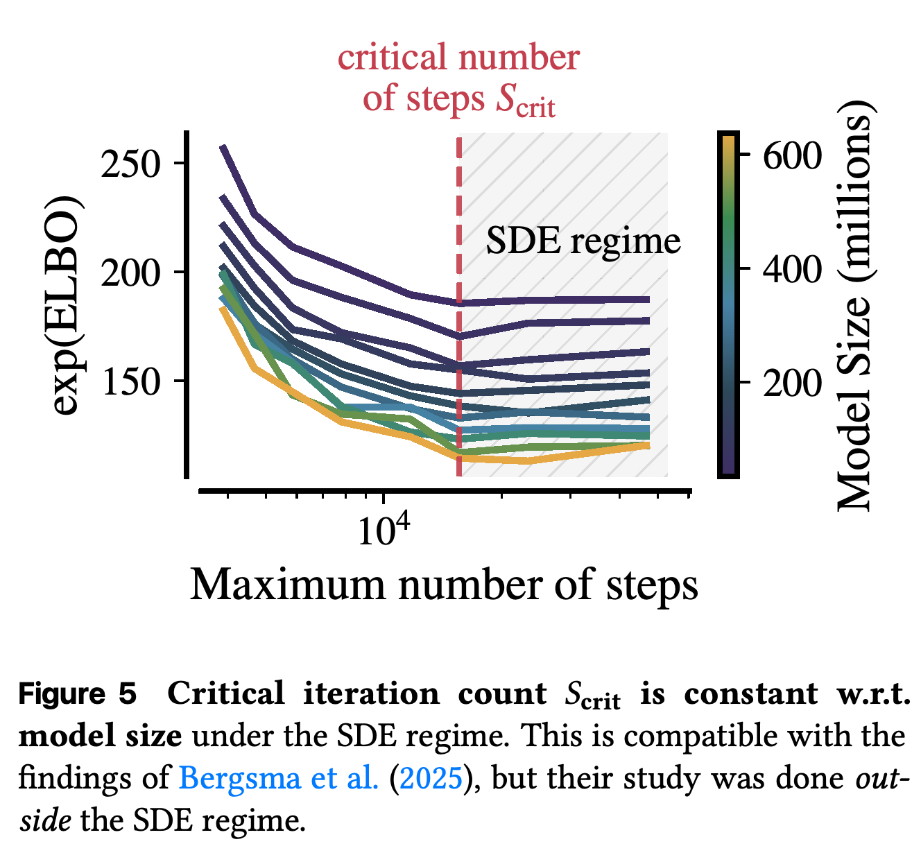
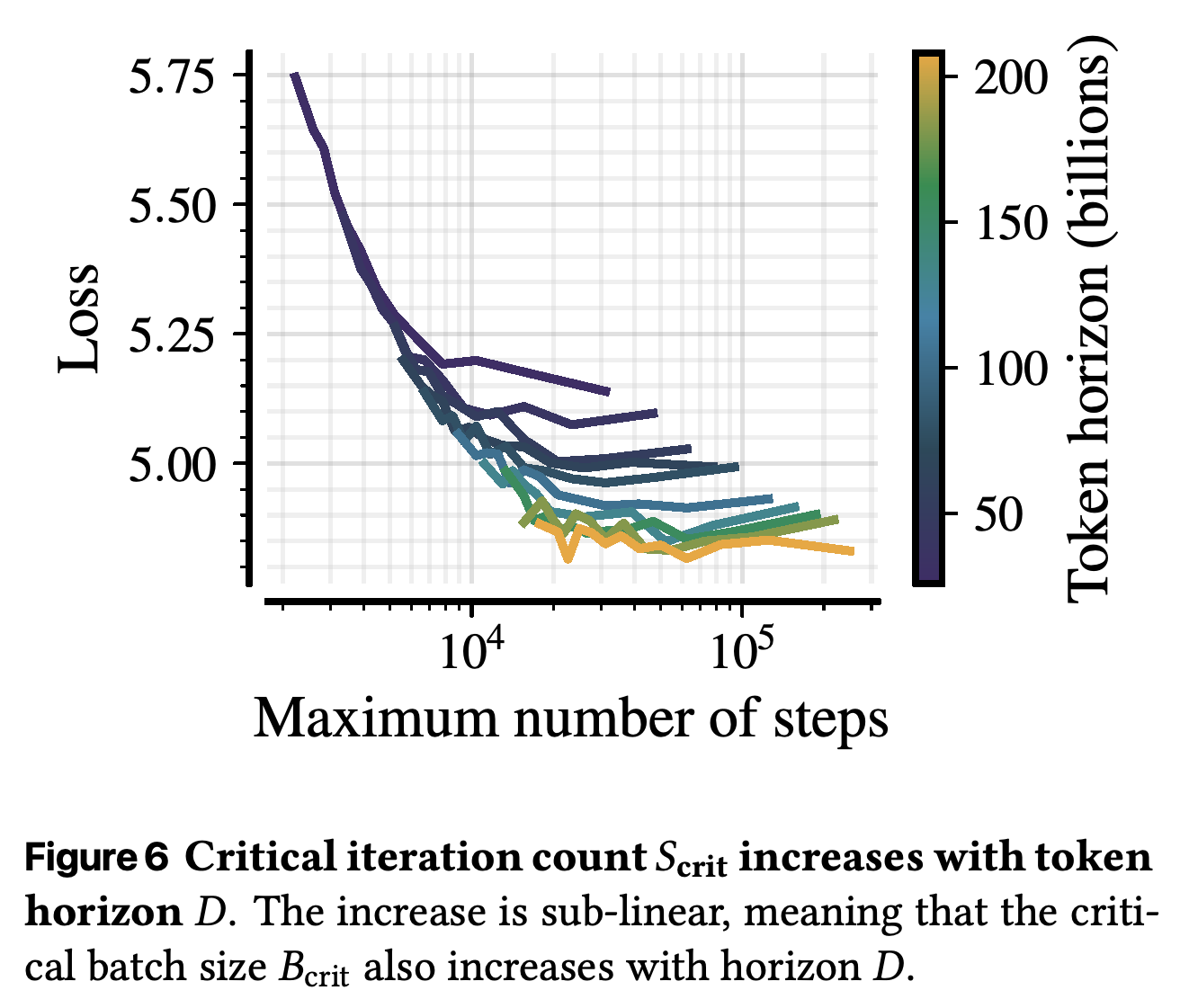
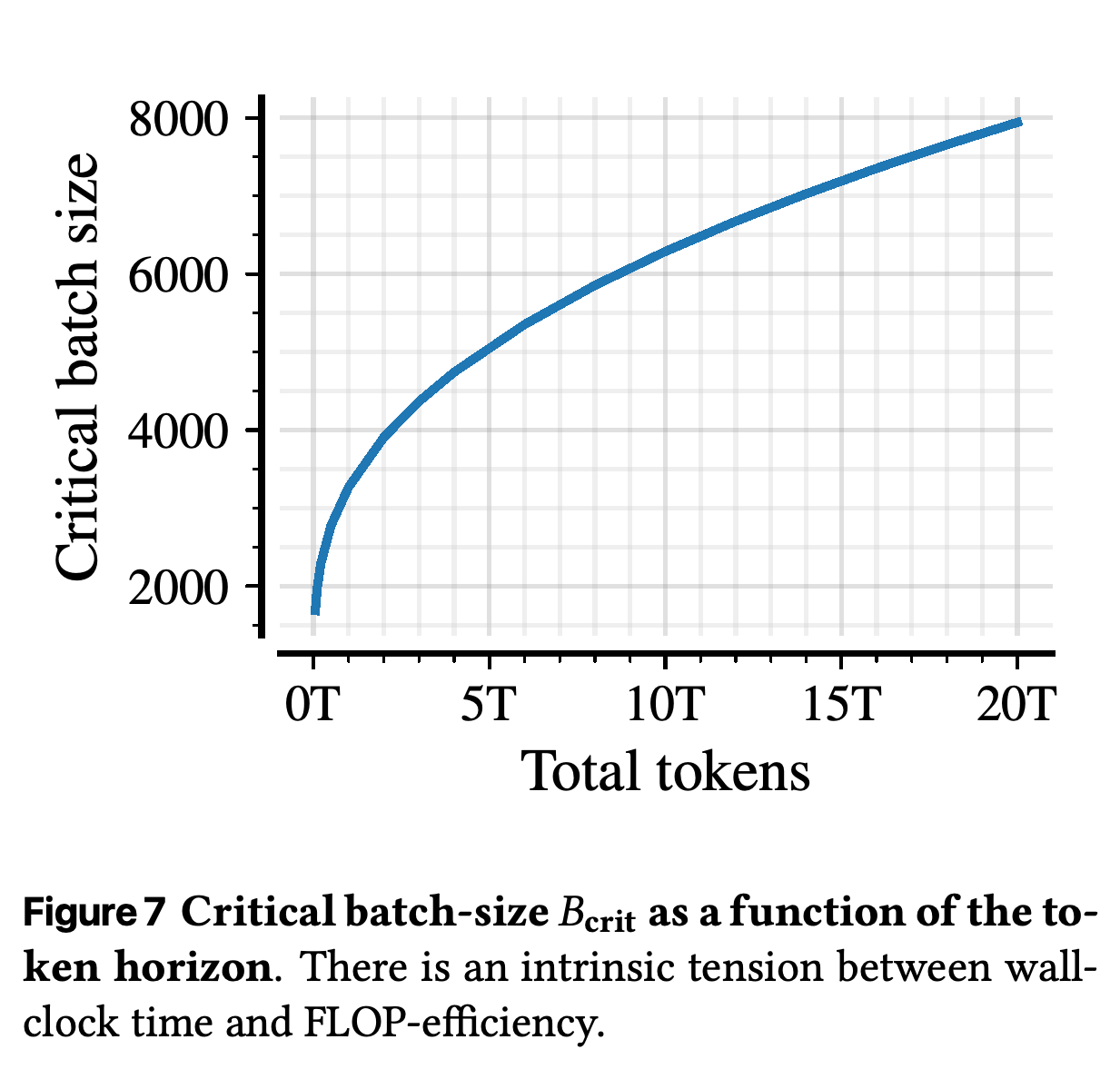
The critical iteration count Scrit is the minimum number of optimizer steps needed to retain FLOP-efficient training, with Bcrit = D/(L Scrit) when batch size is measured in sequences. At a fixed 13B-token horizon, Scrit is approximately independent of model size; increasing the token horizon raises both the critical step count and the allowable critical batch size sublinearly in the reported experiments.

• Figures 5–7 support choosing physical batch size to saturate hardware while remaining below the empirically measured threshold.
• Beyond Bcrit, more aggressive batching sacrifices token efficiency; GPU count therefore cannot grow proportionally with the token budget indefinitely while preserving that efficiency.
• Some prose in Section 5.1 reverses the step-count inequalities. The definition and figures identify S ≥ Scrit, equivalently B ≤ Bcrit, as the loss-preserving regime.

Different model sizes approach their respective loss plateaus at approximately the same iteration threshold for a fixed token budget. This supports transfer of the critical batch-size constraint across the tested model sizes.

Longer token horizons require more optimization steps before loss reaches its plateau. The critical iteration threshold therefore changes with training duration.

The critical batch size grows sublinearly with total tokens. This limits how far increased parallelism can shorten long training runs without reducing token efficiency.

5.2 Optimal Drift–horizon Tradeoffs

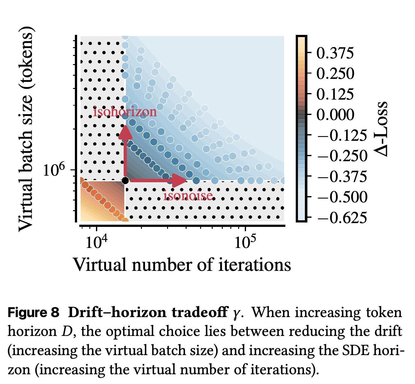
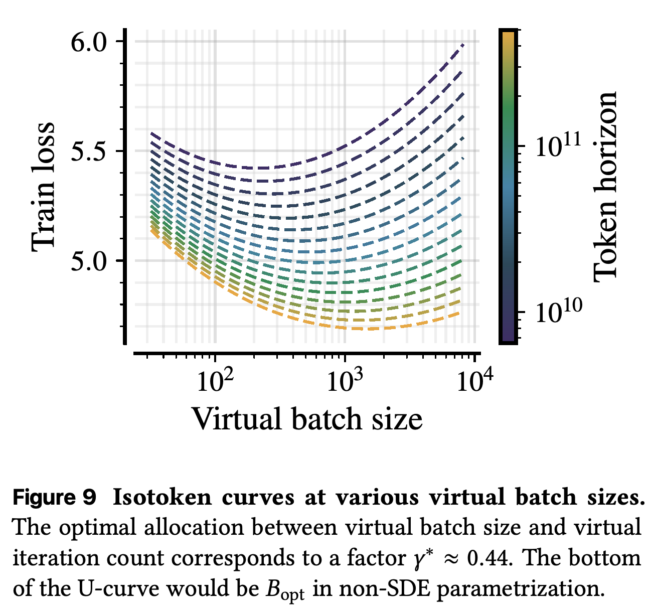
Physical batching is separated from a virtual batch size and virtual iteration count satisfying D = B̃S̃L. A sweep over γ allocates additional tokens between increasing B̃ and increasing S̃, and fitting E + A S̃^−α + B B̃^−β yields α = 0.18, β = 0.23, and γ* ≈ 0.44.

• Figures 8 and 9 show that neither pure isonoise nor pure isohorizon scaling minimizes loss in the tested setup.
• The optimum concerns logical optimization behavior, not a renewed search for hardware batch size.
• The authors note that γ* could change under a different learning-rate schedule, such as warmup-stable-decay.

The loss landscape favors increasing both virtual iterations and virtual batch size rather than following either endpoint direction alone. These virtual quantities describe duration allocation rather than hardware batching.

At each token horizon, the fitted U-shaped curve identifies an intermediate logical batch size. The shifting minima motivate γ* ≈ 0.44 for scaling virtual batching and iteration count together.

5.3 Scaling Laws for Tri-modal MDM

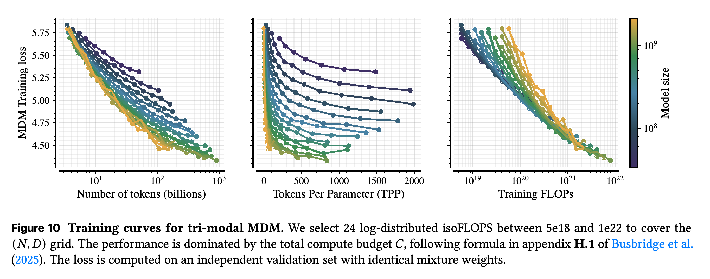
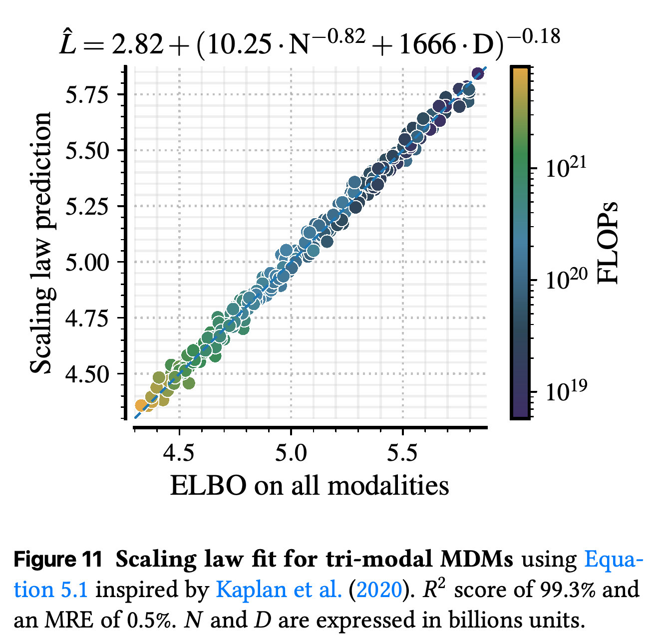
The scaling-law study trains 262 tri-modal MDMs with tokens-per-parameter ratios from 1 to 2000 across 24 logarithmically spaced isoFLOP budgets between 5 × 10^18 and 1 × 10^22. Fitting L(N,D) = E + (A N^−a/b + B D^−1)^b with basin hopping and LBFGS, 20 bootstrap samples, and 90%–10% cross-validation gives a ≈ 0.14, b ≈ 0.17, R² = 99.3%, and mean relative error of 0.5%.

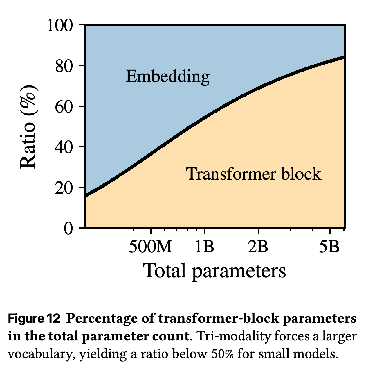
• N in the fitted loss law excludes embedding parameters, whereas training FLOPs include embedding computation but exclude modality tokenizers.
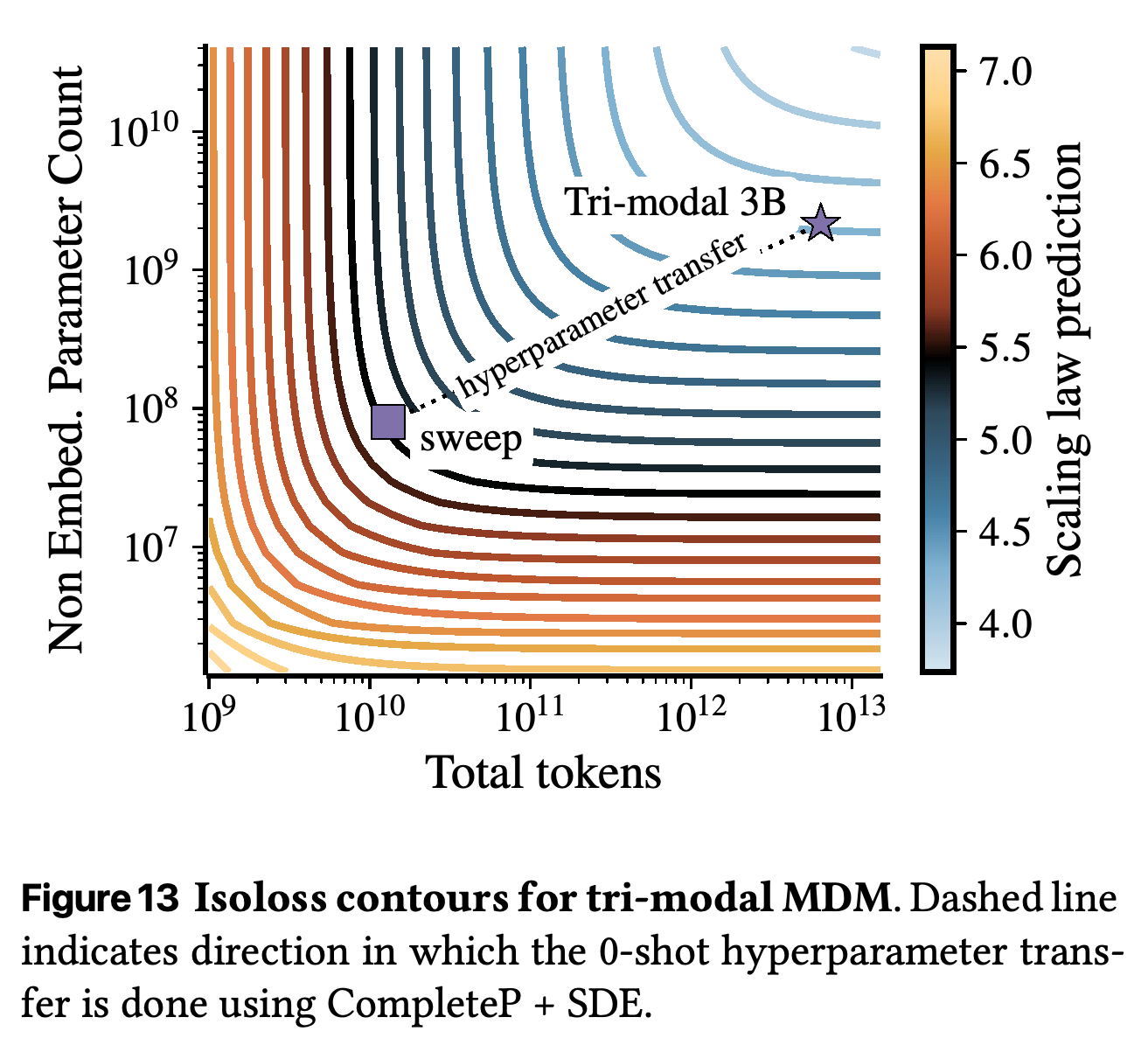
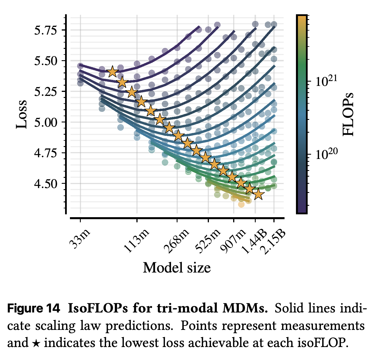
• Figures 10–14 show validation-loss measurements, prediction agreement, embedding overhead, isoloss contours, and the loss-minimizing model size at each compute budget.
• The reported frontier D★(N) = 7754 · N^0.84 implies optimal tokens per parameter proportional to N^−0.16 and approximate compute allocations N★(C) ∝ C^0.55 and D★(C) ∝ C^0.45.

The 262-model measurements align more closely against FLOPs than against token count or tokens per parameter. Although the panels are labeled training loss, the caption specifies an independent validation set with matching mixture weights.

Predicted and measured losses closely follow the diagonal, consistent with the reported R² of 99.3% and mean relative error of 0.5%. The formula printed above the plot differs from Equation (5.1), so the agreement plot does not resolve which displayed expression should be used for reproduction.

Embedding parameters dominate smaller models because the unified vocabulary is large. Total parameter count and non-embedding backbone size are therefore not interchangeable in scaling-law fits or compute accounting.

The contours describe model-size and data combinations predicted to achieve equal loss. The transfer path connects the small tuning model to the longer-trained 3B demonstration, making the extrapolation range explicit.

Each fixed-compute curve has a loss-minimizing model size, marked by a star. The measurements and predictions show the loss penalty from allocating a fixed budget to an excessively small or large backbone.

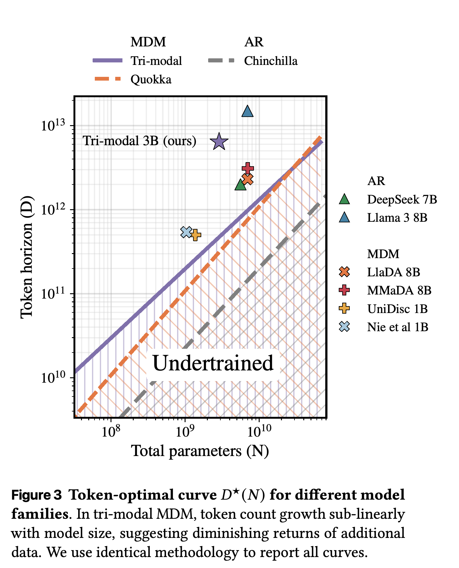
The asymptotic trend does not establish a practical data-efficiency advantage over autoregressive language models. The paper estimates approximately 480B tokens for a 3B model, compared with approximately 60B under the cited Chinchilla rule, and places the crossing with the Quokka diffusion language-model frontier near 20B parameters and approximately 2T tokens.

• Figure 3 compares frontiers using total parameter counts and a common optimization methodology; the showcased 3B model is trained beyond the estimated compute-optimal token horizon.
• Scaling exponents describe relative benefits within a model family, not absolute capability or superiority across families.
• Irreducible loss, model-family bias, forward-process-dependent ELBO bounds, data composition, and repetition complicate cross-family comparisons.

The tri-modal frontier requires more tokens at practical model sizes than the plotted Chinchilla reference, despite its sublinear exponent. The showcased 3B model lies above its estimated compute-optimal frontier; Quokka is shown as another MDM family, not an autoregressive baseline.

6 Data

Except for the mixture ablation, the default tri-modal sampling weights are approximately equal: 33% text-only, 33% image-text, and 33% audio-text. Section 6 describes a token horizon below the total dataset size, with selected small high-quality components repeated up to 4 times; the anti-masking comparison separately uses a two-epoch baseline.

• Text combines Nemotron-CC, DCLM, selected The Pile subsets, licensed StackOverflow, Qwen-32B reasoning-trace synthetic data, and other licensed corpora, with additional privacy and licensing-related filtering.
• Audio comprises 2M hours of web audio transcribed by Whisper and filtered for private information, speech activity, dialogue, production quality, and production complexity.
• Image-text data combines CC3M, CC12M, COYO, recaptioned data, and other licensed datasets used in Manzano. Validation loss uses separate splits with matching mixture ratios.

7 Results

The results evaluate the unified 3B model and independently ablate modality mixing, inference hyperparameters, and anti-masking. Masking-schedule comparisons appear in Appendix F; the ablations start from the same setup rather than combining all interventions cumulatively.

7.1 Unified 3B Tri-modal MDM

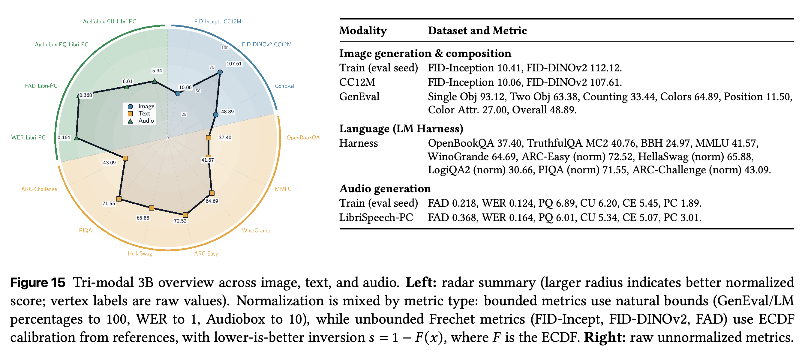
The pretrain-only 3B model is evaluated with LM evaluation harness, image FID using Inception-v3 and DINOv2-L features, GenEval, and speech FAD, WER, and Audiobox Aesthetics. Figure 15 reports CC12M FID-Inception 10.06 and FID-DINOv2 107.61, GenEval overall 48.89, MMLU 41.57, and LibriSpeech-PC FAD 0.368 and WER 0.164.

• GenEval single-object performance is 93.12, but counting is 33.44, position is 11.50, and color attributes are 27.00, indicating uneven compositional performance.
• Language scores include ARC-Easy normalized 72.52, HellaSwag normalized 65.88, PIQA normalized 71.55, and BBH 24.97; the overview does not include a matched autoregressive baseline.
• Speech generation receives reference text and ground-truth duration, so these results do not evaluate autonomous duration prediction.
• The radar chart combines natural-bound normalization with ECDF calibration for unbounded distance metrics; its radii are not directly comparable raw measurements.

The raw metrics show tri-modal functionality with uneven performance, especially on image composition. The radar uses different normalization schemes by metric type, so its geometry should not replace inspection of the numerical results.

7.2 Modality Mixing Ratios

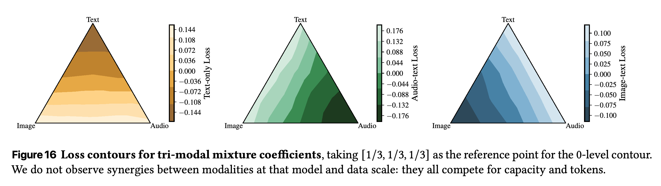
Fifteen mixture experiments use a 320M-parameter model, including 80M non-embedding parameters, trained on 13B tokens, with each modality assigned at least 20% of the mixture. Increasing a modality’s own weight reduces its loss, but changing the relative weights of the other two modalities shows no observable synergy at this scale.

• Figure 16 references loss differences to [1/3, 1/3, 1/3], supporting equal weighting as a balanced default rather than a universally optimal mixture.
• The finding concerns modality-specific validation loss at small scale; it does not rule out larger-scale transfer benefits or task-level synergies.

Each modality’s loss improves mainly toward its own mixture vertex, with differences referenced to equal weighting. At 320M parameters and 13B tokens, the contour structure shows no observable loss synergy from reallocating weight between the other two modalities.

7.3 Best Generation Hyperparameters

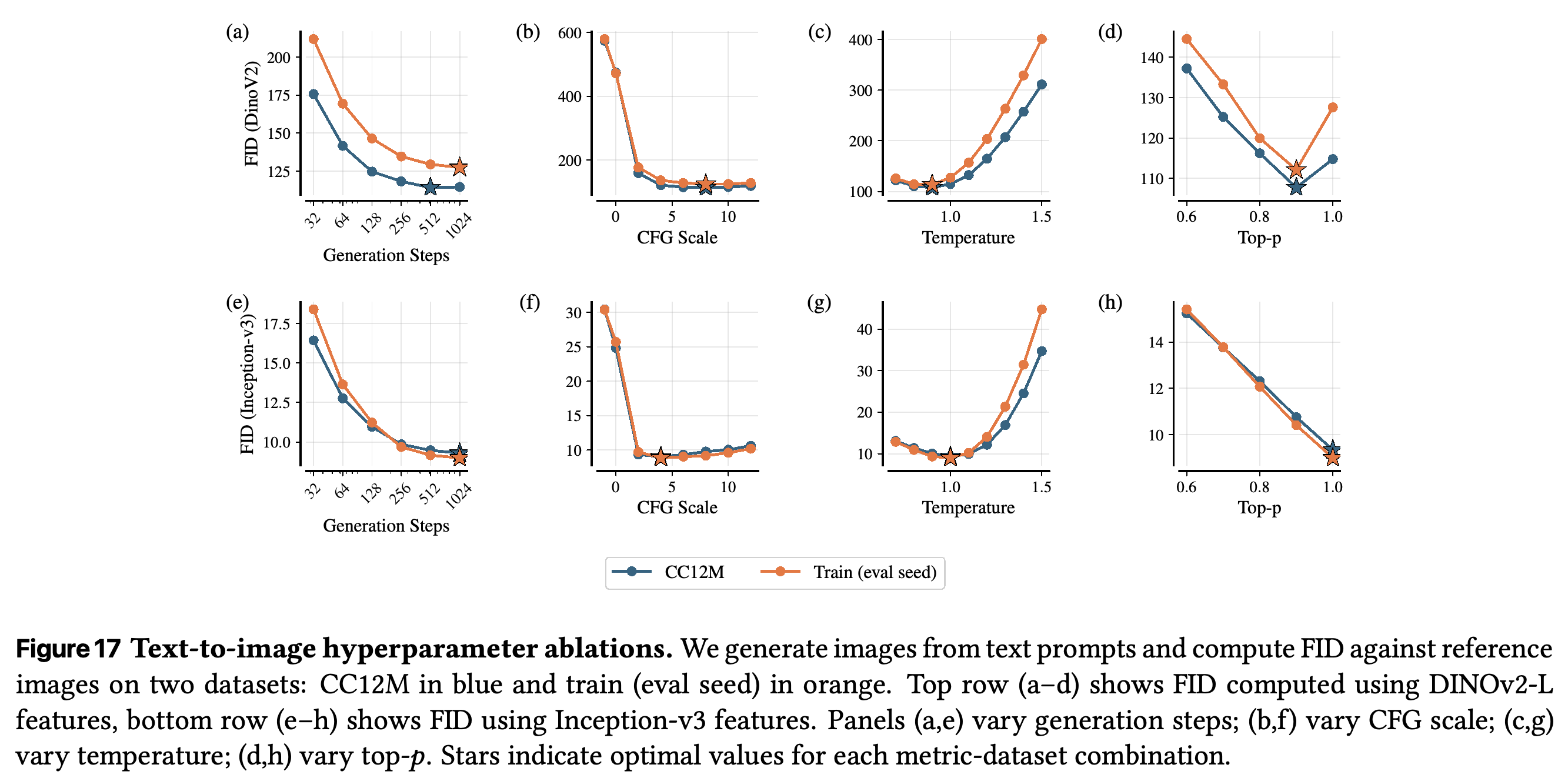
Text-to-image inference sweeps vary CFG, temperature, top-p, and generation steps one at a time using 10,000 images conditioned on CC12M and train (eval seed) prompts. The baseline settings are CFG = 6.0, temperature = 1.0, top-p = 1.0, and 1024 generation steps.

• Figure 17 shows diminishing FID improvements as the number of steps increases.
• Guidance and temperature have interior optima. DINOv2-L FID favors top-p around 0.9, whereas Inception-v3 FID favors 1.0 in the plotted sweeps.
• CFG obtains its unconditional prediction by fully masking the text prompt; these sweeps do not jointly optimize interacting sampling parameters.

More denoising steps improve image FID with diminishing returns, while guidance and temperature have interior optima. DINOv2-L and Inception-v3 favor different top-p values, demonstrating that preferred settings depend on the feature extractor.

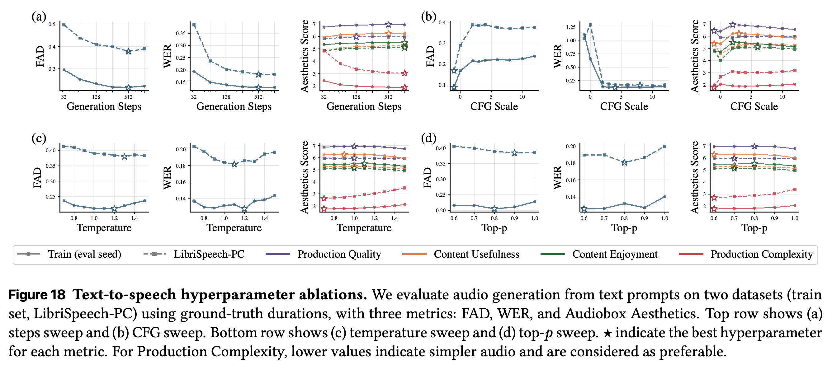
Text-to-speech sweeps begin with 10,000 samples from each of train (eval seed) and LibriSpeech-PC, retain durations ≤ 30 seconds, and supply ground-truth duration for generation. Approximately 70% and 99% of the respective samples remain; baseline settings are CFG = 3.0, temperature = 1.2, top-p = 0.9, and 1000 generation steps.

• Figure 18 shows diminishing returns from additional steps and a guidance trade-off: stronger conditioning improves WER but worsens FAD.
• Temperature, top-p, and CFG have different optima across fidelity, transcription accuracy, and aesthetic dimensions. Lower Production Complexity is treated as preferable in this evaluation.
• Similar trends on LibriSpeech-PC support transfer of the observed sensitivities to an external dataset within the reference-duration protocol.

Guidance improves transcription accuracy while worsening distributional audio fidelity, and sampling optima differ across aesthetic dimensions. The broad trends across the two datasets are measured with supplied reference durations; lower Production Complexity is treated as preferable.

7.4 Anti-Masking

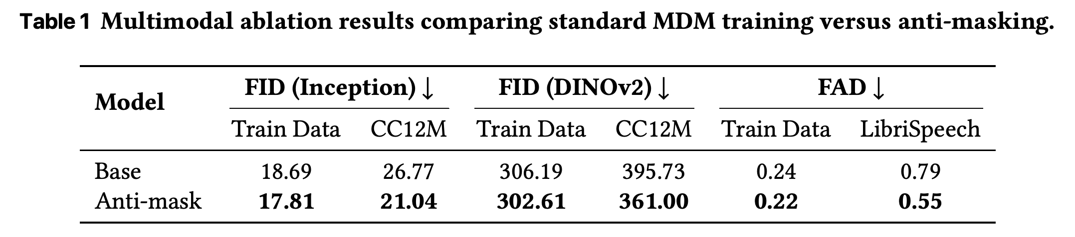
Anti-masking creates two complementary masked versions of each input to reduce training variance. To match computation, the experiment compares one epoch of paired anti-masked examples against two epochs of ordinary masking, using approximately 7B text models at 100 unique tokens per parameter and approximately 1.3B multimodal models at 50 unique tokens per parameter.

• Table 1 shows lower values for all reported image and audio distances: CC12M FID-Inception falls from 26.77 to 21.04, and LibriSpeech FAD falls from 0.79 to 0.55.
• Table 2 improves most language-task means, including BBH from 21.52 ± 0.46 to 27.05 ± 0.50 and MMLU from 30.20 ± 0.39 to 32.86 ± 0.39.
• TruthfulQA declines from 43.12 ± 1.45 to 36.97 ± 1.41, so the benchmark effect is not uniformly positive.
• Compute neutrality applies to this replacement of repeated ordinary examples. Anti-masking still processes two corrupted instances per unique sample.

Anti-masking lowers every reported image FID and audio FAD in the compute-matched comparison. LibriSpeech FAD falls from 0.79 to 0.55, whereas train-data FAD changes from 0.24 to 0.22.

Most language-task means improve, with substantial changes for BBH and ARC-Challenge, but TruthfulQA declines. The reported mean accuracy and standard deviation entries support a mostly positive rather than universal benchmark effect.

8 Conclusion

The conclusion combines a shared discrete tri-modal architecture with empirical guidance for optimization transfer, compute-optimal allocation, and modality-specific sampling. The experiments establish feasibility and training-recipe results without demonstrating superiority over competing generative model families.

• SDE transfer reduces physical batch-size tuning within the critical regime.
• Anti-masking improves most tested outcomes under a compute-matched repetition setup, while inference choices depend on both modality and metric.

Appendix

• A General formulation of weighting and the masking process, A.1 Connection of Loss Weighting and Cumulative Corruption, and A.2 Unbiasedness of the Importance Weighting develop the absorbing-mask transition process, cumulative survival probability, reverse posterior, and time-dependent loss weighting. The derivation changes from −ᾱ′t/(1 − ᾱt) for the posterior rate to ᾱ′t/(1 − ᾱt) for the displayed loss weight, creating a sign inconsistency. The 1/t subsampling argument also treats reconstruction loss as fixed despite its dependence on corrupted context and does not reconcile that argument with the masked-position normalization in Section 3.
• B Tokenizer Ablations and B.1 Audio Tokenizer Ablations compare pretrained DAC, pretrained Higgs Audio v2, and a retrained DAC-style codec under the 3256-token context and 30-second audio constraint. Higgs Audio v2 decoded with four codebooks is selected for its rate–distortion trade-off, with LibriTTS-clean reconstruction PESQ 2.544. More codebooks improve reconstruction but increase sequence length.
• B.2 Image Tokenizer Ablations compares Cosmos, IBQ, OpenMagVIT, UniTok, and MoVQGAN using reconstruction FID on CC12M and ImageNet, including ImageNet at 256 and 512 resolution. MoVQGAN is selected for its balance of reconstruction quality, compression, and vocabulary size: its CC12M rFID is 0.50 with 1024 tokens per image and vocabulary size 16,384.
• C Training details includes C.1 Optimal Global Hyper-Parameter Search, C.2 Runtime as Function of Batch Size, and C.3 Hyperparameters for the Unified 3B Tri-modal MDM. The global search uses 2900 trials at a stated 320M total parameters and 13B tokens, although Figure 19’s caption says 350M; runtime measurements separate GPU saturation from node-count expansion and its communication overhead. The final recipe specifies base learning rate 9e−4, AdamW ε = 1e−8, β1 = 0.9, β2 = 0.95, weight decay 0.1, 2,000 warmup steps, and z-loss weight 1e−5.
• D MDM with Per-module Hyperparameters searches module-specific and depth-dependent optimizer and initialization multipliers on an eight-block, width-1024 model trained on 13B multimodal tokens. It reports a 1.81× reduction in tokens required to reach equivalent loss at the base scale, with larger text embedding and unembedding learning rates and stronger numerical damping in later blocks. Figure 21’s caption labels the model 350M, whereas the surrounding prose states 320M.
• E Extended Scaling Laws Results explains why non-embedding parameter count cannot be substituted directly into C = 6ND for small models with large embedding overhead. Compute-optimal curves use the full FLOPs-per-token calculation; a separate text-only study uses CompleteP without SDE scaling, sequence length 4,096, and model-dependent batches for GPU occupancy. Its fitted form is L̂ = 1.88 + 0.28 · N^−0.48 + 0.75 · D^−0.21.
• F Masking Schedules for Image and Audio Generation compares linear, cosine, polynomial, and geometric schedules by training 1B models for 100k steps with other settings fixed. Image evaluation uses 8,192 samples, 256×256 resolution, 1024 diffusion steps, temperature 0.9, and top-p 0.9; audio evaluation uses 10,000 samples, reference durations, 512 steps, temperature 1.0, and top-p 0.9. Polynomial masking gives the strongest overall results, with reported preferred CFG ranges of 7–9 for images and 1–3 for audio, although the plotted Production Complexity scores do not show uniform polynomial superiority at every guidance scale.
• G Extended generations provides image samples and their complete synthetic-caption prompts. The examples were selected from a larger generation pool using quality filtering and diversity, so the galleries illustrate capabilities rather than typical success rates. H Contributions records responsibilities for code, experiments, data preparation, infrastructure, theoretical formulation, and project leadership.

Brief Thoughts

The clearest practical contribution is the separation of physical batch size from logical optimization dynamics: the measured loss plateau and its failure threshold support hardware-aware batching within a defined regime. The systematic scaling study supplies useful allocation estimates, but those estimates remain specific to the tokenizer, data mixture, architecture, and transfer rules tested. Deployment evidence is limited: sampling uses many steps, no matched inference-latency comparison is reported, and speech generation receives reference durations. The 3B results establish generation across three modalities, while low GenEval position and counting scores limit claims about compositional understanding. Inconsistent formula labels, step-count inequalities, and search-model sizes should be resolved before reproducing the training recipe.