NVIDIA OmniDreams: Real-Time Generative World Model for Closed-Loop Autonomous Vehicle Simulation | Summary

Contents

• Summary
• 1. Introduction
• 2. Data
  • 2.1. Data Sources
  • 2.2. Conditioning Signal Extraction
  • 2.3. Data Curation and Quality Filtering
  • 2.4. Dataset Composition
  • 2.5. Curation and Inspection with SIL-Wheel
• 3. Model Architecture
  • 3.1. Network Architecture
  • 3.2. Consistent Multi-View Generation
• 4. Training
  • 4.1. World-Scenario Control and Multi-view adaptation
  • 4.2. Mid-training for Autoregressive Generation
  • 4.3. Distillation
• 5. Training-free Model Inference Optimization
  • 5.1. Model Optimization
  • 5.2. Multi-GPU Inference
  • 5.3. End-to-End Performance
  • 5.4. FlashDreams: Generalized Inference and Serving Infra
• 6. Closed-Loop Simulation Integration
  • 6.1. AlpaSim
  • 6.2. Networked integration in AlpaSim
  • 6.3. Session-based state
  • 6.4. Supporting chunked generation
• 7. Post-training OmniDreams as a World-Action Model (WAM)
  • 7.1. Architecture and training
  • 7.2. Closed-loop comparison to Alpamayo 1.5
• 8. Post-Training OmniDreams as a Diffusion Fixer
• 9. Experiments and Results
  • 9.1. Simulation Quality
  • 9.2. Long Rollouts
  • 9.3. Long-tail Coverage and Counterfactual Variations
  • 9.4. Closed-Loop Evaluation
• 10. Related Work
  • 10.1. World models for closed-loop AV Simulation
  • 10.2. Closed-loop AV simulation infrastructure
• 11. Conclusion
• Appendix
• Brief Thoughts

This article explains the key points of NVIDIA OmniDreams: Real-Time Generative World Model for Closed-Loop Autonomous Vehicle Simulation.

• 2026-06-02 (arXiv)
• Basant, Aarti, Kar, Amlan, Paschalidou, Despoina, Wei, Fangyin, Ferroni, Francesco, Cobo, Guillermo Garcia, Turki, Haithem, Ling, Huan, Seo, Jaewoo, Lucas, James, et al.
• Paper
• Github
• Project Page

Read this article in Korean

Summary

• OmniDreams adapts Cosmos-Predict 2.5 into an action-conditioned camera simulator for closed-loop autonomous-driving evaluation. It generates short video chunks from a first-frame RGB seed, text, structured simulator state, and cached visual history, supporting visual conditions and viewpoints beyond scene-specific reconstruction coverage.
• Training combines driving-domain and multi-view adaptation, causal Diffusion Forcing, and two-step Self Forcing with Distribution Matching Distillation (DMD). Inference optimizations achieve 68 effective FPS for one camera on one GB300 and 105 effective FPS per camera for four cameras on 16 GB300 GPUs at 704 × 1280; these measure chunk-generation throughput, not policy replanning rates.
• On 1,000 held-out clips, Self Forcing improves single-view FVD from 31.7 for the causal Diffusion Forcing model to 24.8, although Temporal Sampson worsens from 1.87 to 1.90. Progressive long-context distillation reduces mean segmented FVD on 20-second rollouts from 240.0 to 179.4, but quality still deteriorates across successive windows.
• A controlled 501-scene comparison preserves the aggregate incident ranking of four policy configurations when switching between NuRec and OmniDreams, despite differences in absolute incident rates. A separate preliminary 574-scene experiment reduces collisions from 6.9% for Alpamayo 1.5 to 4.2% for an approximately 2 B-parameter OmniDreams World-Action Model; neither experiment establishes real-world safety equivalence.

1. Introduction

Closed-loop evaluation requires observations to change with policy actions rather than replaying a fixed recording. Reconstruction-based neural simulators support controlled variations within captured scenes, but novel viewpoints, weather, articulated objects, and scene content can exceed their reconstruction coverage. OmniDreams uses a generative visual prior for sensor synthesis while retaining AlpaSim as the state-update and orchestration layer.

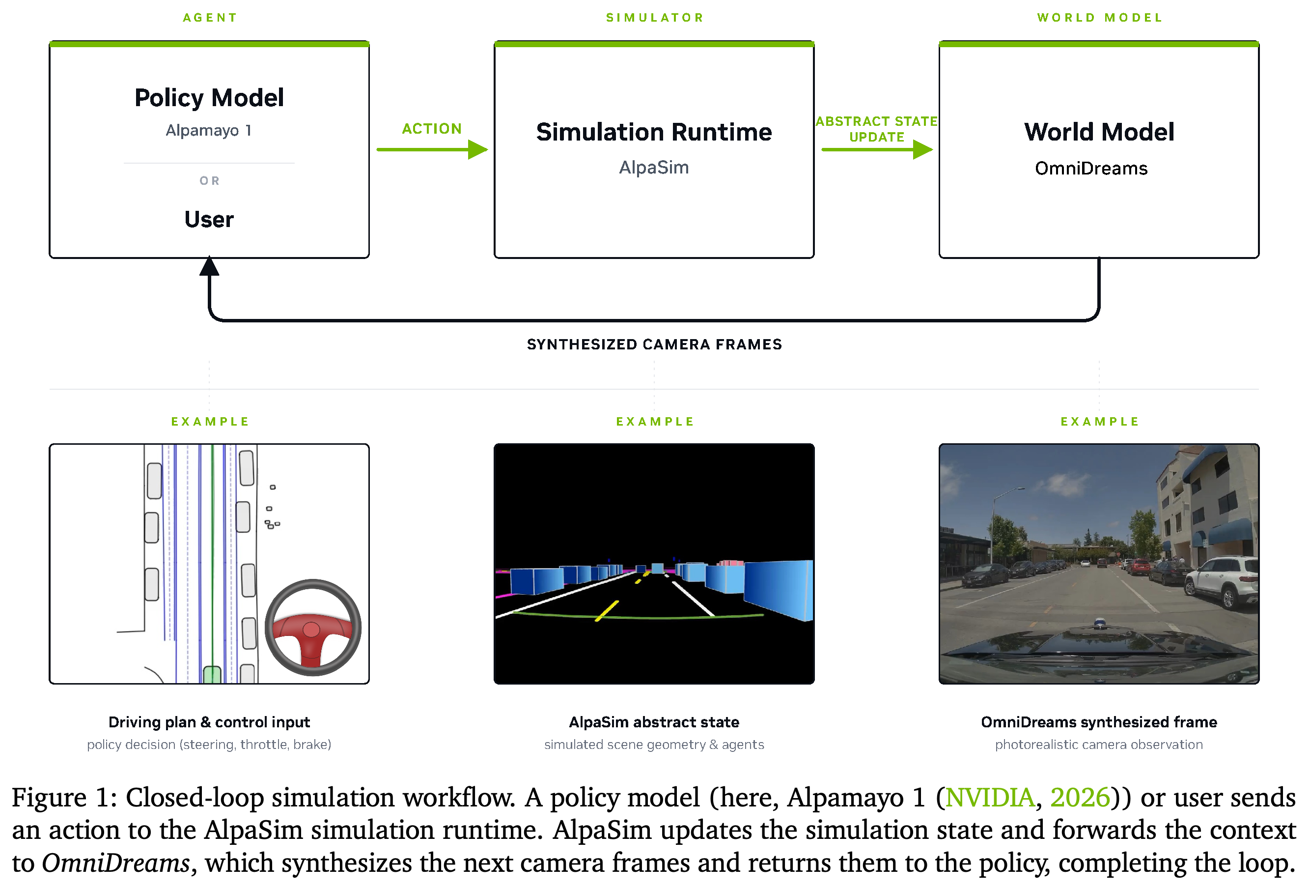
• Figure 1 separates the policy, simulation runtime, and sensor generator: an action updates AlpaSim’s abstract state, and OmniDreams returns camera observations for the next policy decision.
• The report examines two uses of the learned backbone: a real-time camera renderer and a post-trained trajectory-prediction policy.

The feedback arrow makes the causal dependency explicit: the policy changes simulator state before new camera observations are synthesized. OmniDreams supplies sensor images rather than replacing the runtime’s state, traffic, and physics responsibilities.

2. Data

The data pipeline pairs driving video with structured scene representations, ego trajectories, and textual descriptions. These inputs train the model to generate temporally consistent observations aligned with simulator-controlled geometry and motion.

2.1. Data Sources

Mid-training uses Real Driving Scene (RDS), comprising 3M 20s clips, while finetuning and post-training use RDS-HQ-1M, an expanded quality-focused corpus with approximately 1.14M 10s/20s clips. Both originate from driving logs across 15 countries and contain 1080p video at 30 FPS from seven synchronized cameras: front-wide, front-telescope, front-left, front-right, rear-left, rear-right, and rear-tele.

• RDS balances road environment, daytime/nighttime conditions, and driving speed; it is also included in Cosmos-Predict 2.5-AV pre-training.
• RDS-HQ-1M emphasizes visual quality and accurate world-scenario annotations.

2.2. Conditioning Signal Extraction

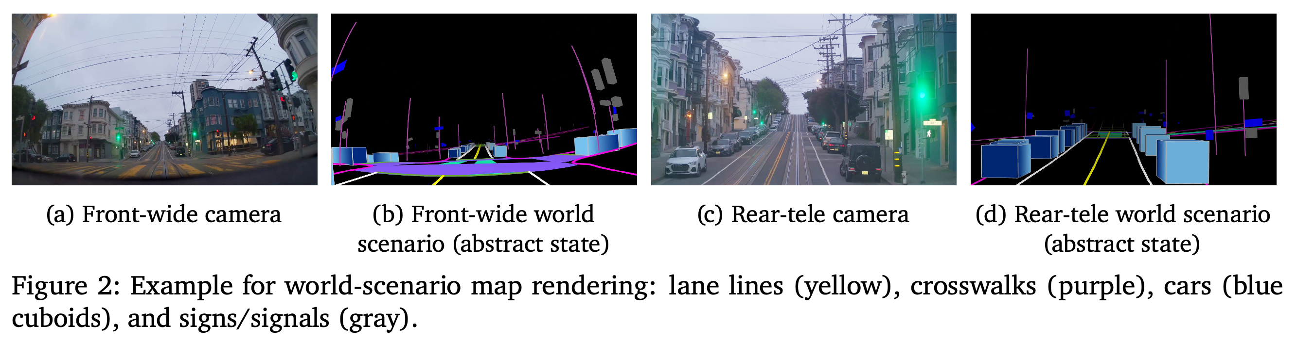
World-scenario map. Static HD-map elements and tracked dynamic actors are projected into each camera using its calibration, producing pixel-aligned lines, surfaces, and shaded cuboids. Text prompts. Qwen2.5-VL-7B describes scenery, weather, driving behavior, and traffic independently for each camera over 10s windows, providing appearance conditioning separate from the geometric control inputs.

• City-level HD maps supply lane lines, road boundaries, stop lines, poles, crosswalks, road markings, traffic lights, and traffic signs; 3D detection and tracking run at 10 FPS and are interpolated to 30 FPS.
• World-scenario rendering incorporates ego actions through the camera trajectory, so action conditioning is mediated by the simulator’s rendered state.
• Short, medium, and long captions contain approximately 40, 80, and 200 words and are sampled with probabilities 0.1/0.2/0.7 during training.

Paired RGB and abstract-state renderings show how camera calibration aligns sparse geometric conditions with target images. Colored lane lines, crosswalks, cuboids, and signs constrain structure without specifying the full photorealistic appearance.

2.3. Data Curation and Quality Filtering

Filtering removes unreliable sensor sequences, uncertain annotations, and prediction disagreements before training. A VLM screens camera footage for artifacts such as chromatic aberration, and ego-trajectory plus visual-feature deduplication down-samples repetitive sequences such as straight highway driving.

2.4. Dataset Composition

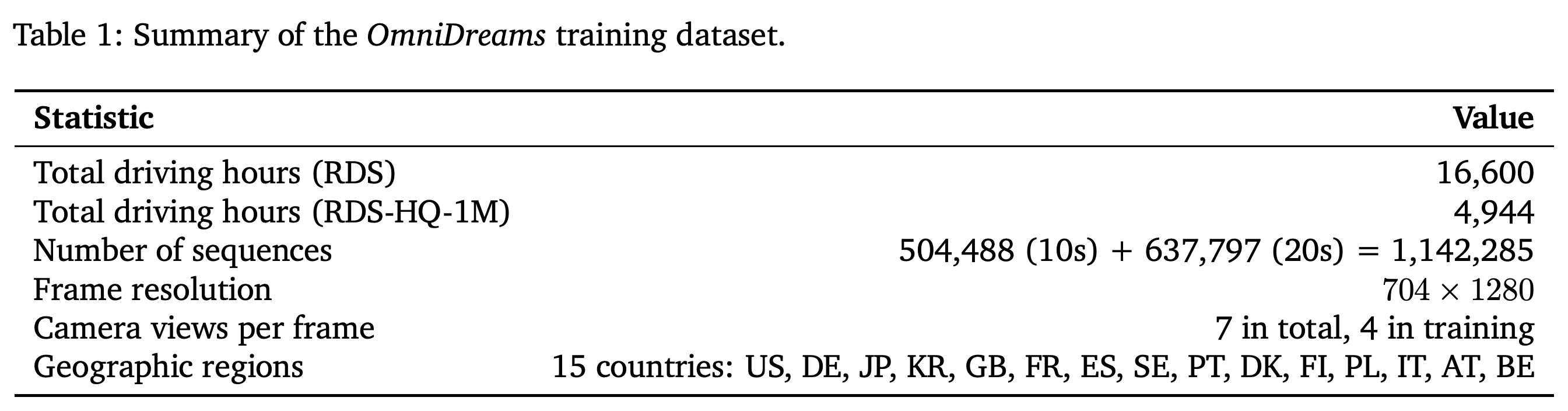
RDS contributes 16,600 h, and RDS-HQ-1M contributes 4,944 h with 1,142,285 clips: 504,488 of 10 s and 637,797 of 20 s. The training resolution is 704 × 1280, with four camera views used from seven available views. The authors hold out 5,000 scenario-balanced clips and obtain 60 s versions of 300 of them for long-term consistency evaluation.

• Held-out categories include vulnerable road users, large vehicles, rain, snow, fog, night, tunnels, railroad crossings, construction zones, and accident scenes.
• Table 1 lists geographic coverage as US, DE, JP, KR, GB, FR, ES, SE, PT, DK, FI, PL, IT, AT, and BE.

The table distinguishes the 16,600 h mid-training corpus from the 4,944 h post-training corpus and records the exact 10s/20s clip composition. Seven recorded views are available, but four are used in training.

2.5. Curation and Inspection with SIL-Wheel

SIL-Wheel provides clip-level search and inspection across the underlying corpora. It combines caption search, semantic and visual retrieval, ego-trajectory queries, classifier scores, and perception filters to construct training mixtures and held-out scenario slices.

• Finetuning slice construction retrieves and upweights underrepresented conditions, including rare weather, construction, vulnerable road users, articulated motion, and complex interactions.
• Eval-set slice construction uses the same interface to create scenario-aware buckets.
• Data inspection checks autolabel quality, triages clips flagged by filtering, and verifies that retrieved slices match their intended conditions.

3. Model Architecture

OmniDreams uses causal, block-autoregressive diffusion to generate observations after each simulator-state update. OmniDreams-SV produces 8 RGB frames per step, corresponding to 2 latent frames, while OmniDreams-MV jointly produces 16 RGB frames per camera, corresponding to 4 latent frames, across four synchronized views. A streaming KV cache reuses past attention representations instead of recomputing the full rollout.

3.1. Network Architecture

The causal transformer combines noisy visual latents with a clean first-frame latent, text encoded through the Cosmos text encoder, world-scenario conditioning, and cached history. A lightweight MLP converts structured control inputs into compact tokens aligned with the visual representation and concatenated with visual tokens, avoiding a separate ControlNet-style network.

• The first RGB image initializes the simulation session; subsequent chunks use updated structured conditions and the evolving memory cache.
• Text enters through cross-attention and conditions lighting, weather, and time of day, while projected maps and actor boxes constrain driving-relevant structure.
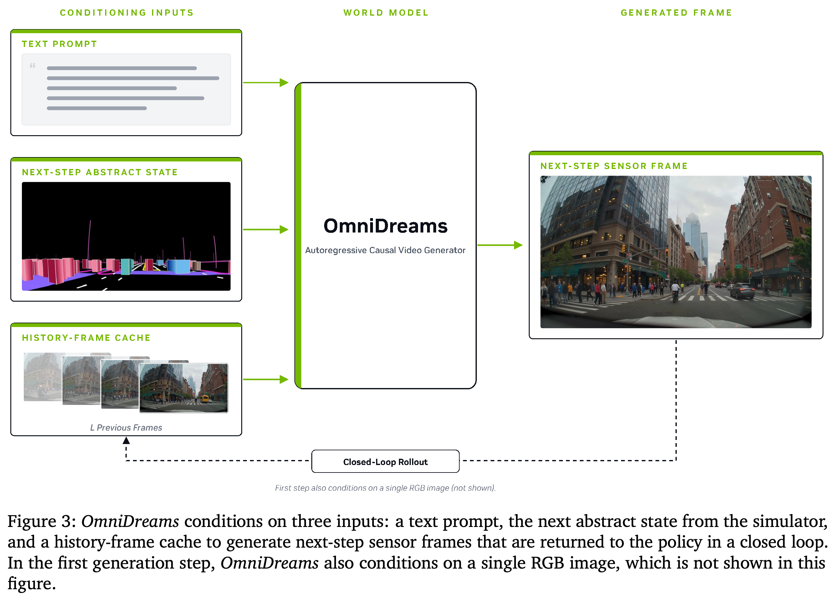
• Figure 3 shows how generated observations become the history used for later generation.

The diagram separates appearance conditioning through text, geometry and motion conditioning through abstract state, and temporal context through cached history. The initial RGB seed is an initialization condition, not a new image required at every step.

3.2. Consistent Multi-View Generation

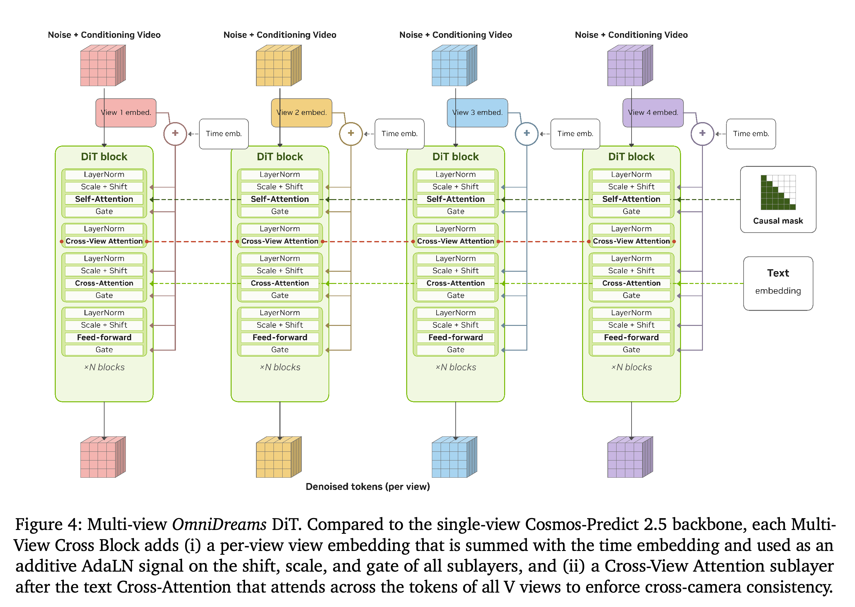
Multi-view generation assigns each camera a learnable view embedding and its own text, seed image, and camera-aligned world-state inputs. Temporal attention operates independently within each view, while cross-view attention exchanges information across cameras at the same time step. The paper reports reducing attention complexity from O(N²T²) to O(NT²) + O(N²), where N is the number of views and T is temporal length.

• This factorization separates temporal modeling from cross-camera correspondence instead of applying unrestricted joint attention over all view-time tokens.
• The architecture is described as supporting up to seven synchronized views, but reported real-time multi-view deployment uses four.
• Figure 4’s drawn sublayer order differs from its caption and Section 4.1, which place cross-view attention after text cross-attention.

Parallel camera streams exchange information through cross-view attention while retaining view identity and causal temporal processing. The drawing places cross-view attention before text cross-attention, whereas the caption and Section 4.1 place it afterward.

4. Training

Training proceeds from driving-domain adaptation of Cosmos-Predict 2.5 to multi-view adaptation for OmniDreams-MV, causal conversion with Diffusion Forcing, and world-scenario control training for both bidirectional teachers and causal students. Self Forcing DMD then distills the causal generator to few-step inference while training it on self-generated context.

4.1. World-Scenario Control and Multi-view adaptation

Preamble. The model uses rectified-flow training with x_t = (1 − t)x + tε, target velocity v_t = ε − x, and L = E_{x,t}[‖u_θ(x_t, t) − v_t‖²], with auxiliary conditioning c for text, first-frame images, and control. Multi-view adaptation first learns camera-specific embeddings on a uniform mixture of four views, then adds cross-view attention and trains jointly on synchronized videos. World-scenario map control adds a zero-initialized control branch and expands training from 93-frame to 189-frame clips.

• The rectified-flow formulation samples ε from N(0, I) and t ∈ [0, 1] from a logit-normal distribution.
• View embeddings enter through adaptive layer normalization; both the embeddings and cross-view output projections are zero-initialized.
• A 1:1 mixture of text-to-video and image-to-video tasks preserves novel-content generation while learning first-frame conditioning; the controlled bidirectional models serve as distillation teachers.

4.2. Mid-training for Autoregressive Generation

Causal Masking factorizes a video as p(x^{1:T}) = ∏_{i=1}^{T} p(x^i | x^{<i}) and restricts attention to the current and previous frames, with a block-autoregressive extension implemented using Flex-Attention. Diffusion Forcing assigns independently sampled noise levels to frames and trains the causal model to predict flow velocities in one parallel forward pass. Training first uses RDS without map control, then adds the control branch and continues on RDS-HQ-1M because causal conversion benefits from more data than the labeled control corpus provides.

• For per-frame timestep vector t, the noisy sequence is x_t^{1:T} = (I − t) · x^{1:T} + t · ε and the velocity target is v_t = ε − x^{1:T}.
• Equation (1) is L_DF = E_{x^{1:T},ε}[‖u_θ(x_t^{1:T}, t) − v_t‖²]. This subsection specifies a log-normal timestep distribution, whereas Section 4.1 specifies logit-normal sampling.
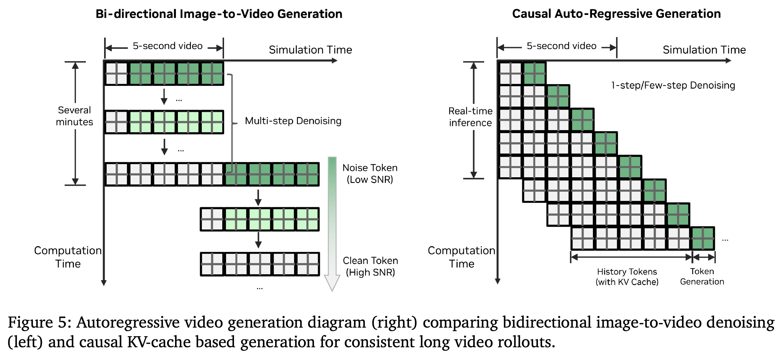
• Figure 5 contrasts bidirectional clip denoising with causal generation that retains previously computed history in the KV cache.

The causal design reuses past tokens as cached context and generates only a short future block. The bidirectional alternative denoises larger clips before observations become available, illustrating the latency motivation for causal generation.

4.3. Distillation

Self Forcing Training via Self-Rollout. Training conditions each generated frame on earlier model outputs, using K=2 denoising steps with schedule [1000, 450], rather than clean ground-truth history. Holistic Distribution Matching via DMD. A frozen real score network and a learned fake score network provide video-level distribution-matching supervision instead of paired pixel reconstruction. Progressive Training with a Longer Teacher. Continued distillation from a longer-context bidirectional teacher reduces shifting artifacts that remain after short-context distillation.

• Backpropagation is restricted to a randomly sampled denoising step, gradients are detached from previous-frame KV embeddings, and training attention matches the rolling inference window.
• Equation (2) uses L_DMD(θ) = E[½‖x̂ − sg[x̂ − (f_ψ(x̂_t, t) − f_φ(x̂_t, t))]‖²], where f_φ is frozen, f_ψ estimates the generated distribution’s score, and sg denotes stop-gradient; the objective targets reverse KL divergence between generated and real-data distributions.
• Distillation uses a curated 58k-video subset emphasizing demanding urban scenes. The longer teacher improves long-horizon quality but does not eliminate degradation in the segmented-FVD results.

5. Training-free Model Inference Optimization

The deployment optimizations leave the distilled diffusion-model weights unchanged. The reported system generates an 8-frame single-view chunk in 118 ms on one GB300 and a 16-frame four-view chunk in 151 ms on 16 GB300 GPUs, both at 704 × 1280.

5.1. Model Optimization

Local temporal attention. Inference retains a window of 6 latent frames, or 24 RGB frames, for OmniDreams-SV and 8 latent frames, or 32 RGB frames, for OmniDreams-MV. Streaming static-shape KV cache. Preallocated cache tensors retain fixed shapes, with updates moved to a separate thread. Compile and CUDA Graphs. Static shapes enable torch.compile and lazily captured CUDA Graph replay across subsequent chunks and rollouts of the same shape.

• Lightweight encoders and decoders. OmniDreams-SV uses LightVAE for conditioning encoding, OmniDreams-MV uses pixel shuffle with negligible encoding latency, and both use LightTAE for RGB decoding.
• Hoisting step-invariant operators. RoPE frequencies are computed once per chunk, and patchify/unpatchify run at chunk entry and exit rather than at every denoising step.
• Table 5 measures the quality cost of the LightTAE decoder used in the low-latency configuration.

5.2. Multi-GPU Inference

Hierarchical context parallelism shards the DiT along camera-view V, temporal T, and spatial HW axes, prioritizing V → T → HW. The 16-GPU four-view deployment uses V=4, T=4, HW=1, exhausting view and within-chunk temporal parallelism before spatial sharding. An in-house ring-attention implementation overlaps KV-shard communication with local attention computation.

• View sharding preserves per-camera self-attention calls and gives close-to-linear scaling until the four-camera axis is saturated.
• Temporal sharding is preferred next because it preserves the per-time-step cross-view attention block, whereas spatial sharding splits both self- and cross-view attention.

5.3. End-to-End Performance

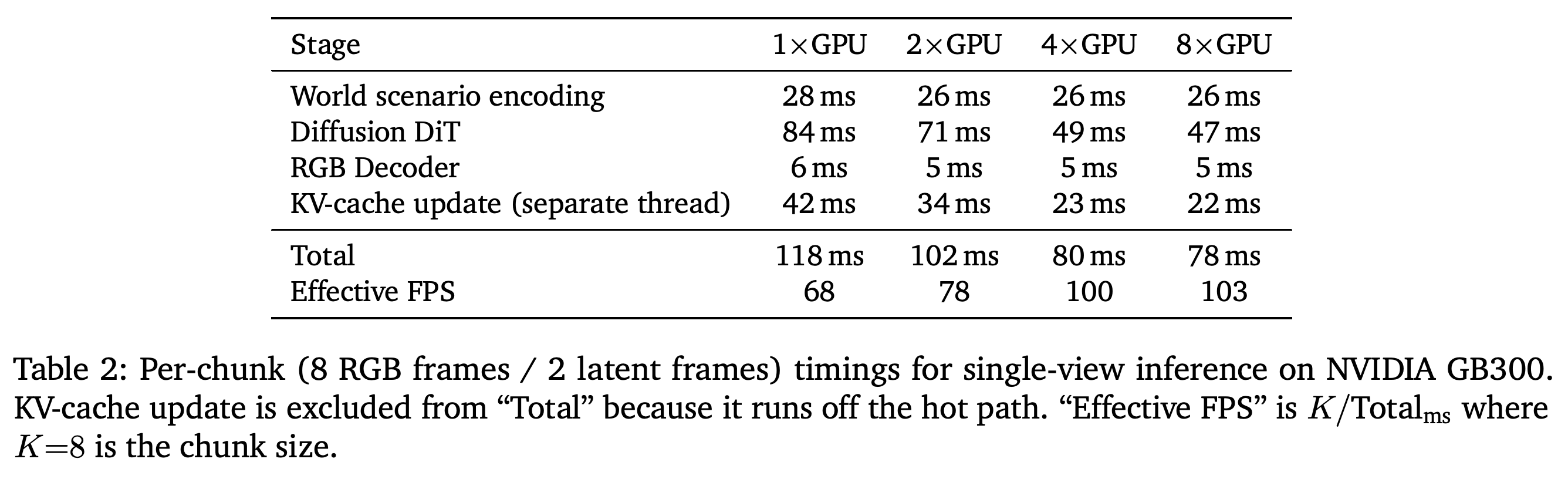
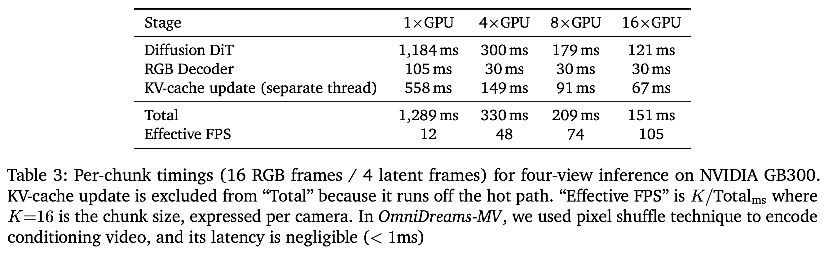
Tables 2 and 3 benchmark the two-step model at 704 × 1280, excluding off-hot-path KV-cache updates from total latency. Single-view inference reaches 68, 78, 100, and 103 effective FPS on 1, 2, 4, and 8 GPUs; four-view inference reaches 12, 48, 74, and 105 effective FPS per camera on 1, 4, 8, and 16 GPUs. The paper defines real-time rendering as 30 FPS.

• Single-view total chunk latency is 118, 102, 80, and 78 ms, with diminishing returns beyond four GPUs as conditioning encoding becomes a substantial fixed cost.
• Four-view total chunk latency is 1,289, 330, 209, and 151 ms; the DiT component falls from 1,184 ms to 121 ms between one and 16 GPUs.
• Effective FPS measures generated frames divided by chunk time. The closed-loop comparison replans every 533 ms, so rendering throughput is not the frequency of feedback control.

Single-view throughput increases from 68 FPS on one GB300 to 103 FPS on eight, but total chunk latency improves only from 80 ms to 78 ms between four and eight GPUs. World-scenario encoding remains 26 ms in those configurations, while cache updates are excluded because they run off the hot path.

Four-view total latency decreases from 1,289 ms on one GPU to 151 ms on 16, yielding 105 effective FPS per camera. The DiT dominates the one-GPU configuration, and pixel-shuffle conditioning encoding contributes less than 1 ms.

5.4. FlashDreams: Generalized Inference and Serving Infra

FlashDreams packages local-window attention, static-shape streaming caches, CUDA Graph execution, and networked serving into an open-source inference stack. Beyond OmniDreams, the authors report up to 1.95× speedup for Wan2.1-based Self Forcing on one GB200 and up to 2.49× for Lingbot-World on four H100s.

• The serving stack provides gRPC and webRTC protocols for streaming control inputs to the server and RGB frames to clients.
• The repository is https://github.com/NVIDIA/flashdreams; the reported speedups are configuration-specific maxima.

6. Closed-Loop Simulation Integration

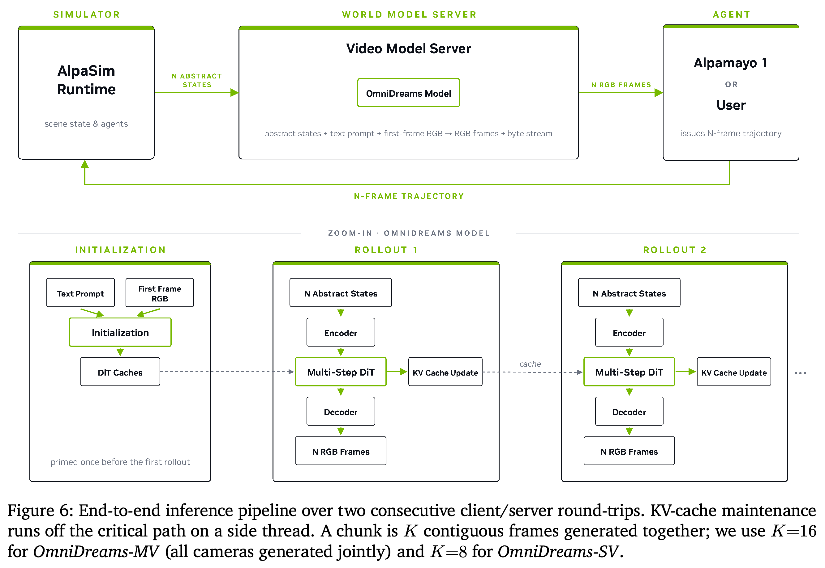
A stateful video-model server connects to the simulator through gRPC. Requests supply trajectories and prompts, with the initial RGB seed sent only at session initialization; the server renders conditions, performs two causal denoising steps, and returns JPEG-encoded frames. KV caches, captured CUDA Graphs, and renderer state persist across chunks.

• Figure 6 shows initialization and two successive round-trips, with cache maintenance separated from the critical rendering path.
• Integration accommodates distributed inference, ordered autoregressive state, and trajectories committed for an entire generated chunk.

Initialization primes persistent state once; later requests encode new abstract-state chunks, run the DiT, and decode RGB while cache maintenance runs on a side thread. Model-side state persists across network round-trips without repeated seed-image transmission.

6.1. AlpaSim

AlpaSim is a research-oriented AV simulator built from Docker-deployed microservices communicating through gRPC. Its asynchronous runtime pipelines concurrent rollouts across specialized services. Integrating OmniDreams replaces the NuRec camera renderer and extends the runtime and protocols to support stateful chunk generation.

• Services must distinguish rollout state across concurrent, potentially out-of-order requests.
• The open-source simulator is available at https://github.com/NVlabs/alpasim.

6.2. Networked integration in AlpaSim

A gRPC server on rank 0 receives simulator requests and forwards rendering work to the remaining distributed ranks through NCCL events. Generated frames are gathered on rank 0, serialized, and returned to AlpaSim, keeping the model’s dependencies and rank-parallel execution separate from other simulator components.

• RDMA-based gRPC or NCCL bulk-frame transfer with gRPC coordination is proposed as future work, not demonstrated in the current integration.
• Those transport changes would address the complexity and lossiness of the existing frame encoding and decoding.

6.3. Session-based state

Each rollout creates a session containing the seed frame, world-map representation, and a preallocated KV cache. The server returns a fresh session ID, which AlpaSim attaches to subsequent requests to select the correct autoregressive history.

6.4. Supporting chunked generation

Chunk generation requires ego and actor poses for every frame before rendering begins, preventing policy or traffic trajectories from changing midway through that chunk without invalidating it. 6.4.1. Post-fetch generation advances policy and traffic using stale visual inputs and inserts generated observations afterward. 6.4.2. Pre-fetch generation, implemented in AlpaSim, predicts and commits multi-step trajectories at chunk boundaries before requesting video.

• Post-fetch requires policies that tolerate visual observations lagging behind egomotion and introduces out-of-order simulation events.
• Pre-fetch interpolates committed trajectories at frame timestamps and injects returned frames as timestamped events, preserving event order.
• Smaller chunks and eventual frame-at-a-time generation are future goals; current chunk semantics limit within-chunk responsiveness.

7. Post-training OmniDreams as a World-Action Model (WAM)

The World-Action Model (WAM) experiment tests whether generative driving representations can support policy prediction. It initializes from the approximately 2 B-parameter OmniDreams-SV causal checkpoint before world-scenario control finetuning and predicts a 6.4-second trajectory at 10 Hz, comprising 64 waypoints.

• The backbone’s front-wide view has a 120° field of view.
• Unlike sensor simulation, trajectory prediction does not require world-scenario map control.

7.1. Architecture and training

WAM adds projected patch features from a DINOv2 (dinov2_vitb14)-initialized encoder and a 30° front-telescope camera, plus a history token encoding 1.6 s of ego motion. The history token attends to current and past video tokens but not other history tokens; its output conditions a 12-layer U-Net-shaped MLP flow model over a trajectory latent in R^{64×3}. Joint training sums video and trajectory flow-matching losses with independently sampled noise times.

• The attention mask retains causal video-to-video attention while adding one-way information flow into history tokens.
• Inference runs the DiT once with 4 low-noise video latent frames and one history token, then uses 4 flow-matching steps in the lightweight trajectory MLP.
• No video denoising rollout is required when only the future trajectory is requested.

7.2. Closed-loop comparison to Alpamayo 1.5

Under the original Alpamayo 1.5 evaluation protocol, WAM is evaluated with 10 Hz replanning and 20-second rollouts on 574 Physical AI Autonomous Vehicles NuRec scenes after excluding WAM training scenes. Collision falls from 6.9% to 4.2%, with Front decreasing from 1.0% to 0.9%, Lateral from 0.6% to 0.4%, and Rear from 5.3% to 3.0%, despite approximately 2 B versus 10 B parameters.

• The largest reported directional reduction is in rear collisions.
• These preliminary results support the backbone’s usefulness for policy prediction, but do not isolate representation learning from differences in architecture, training, and conditioning.
• This 574-scene, 10 Hz protocol is distinct from the 501-scene simulator comparison with 533 ms replanning in Section 9.4.

8. Post-Training OmniDreams as a Diffusion Fixer

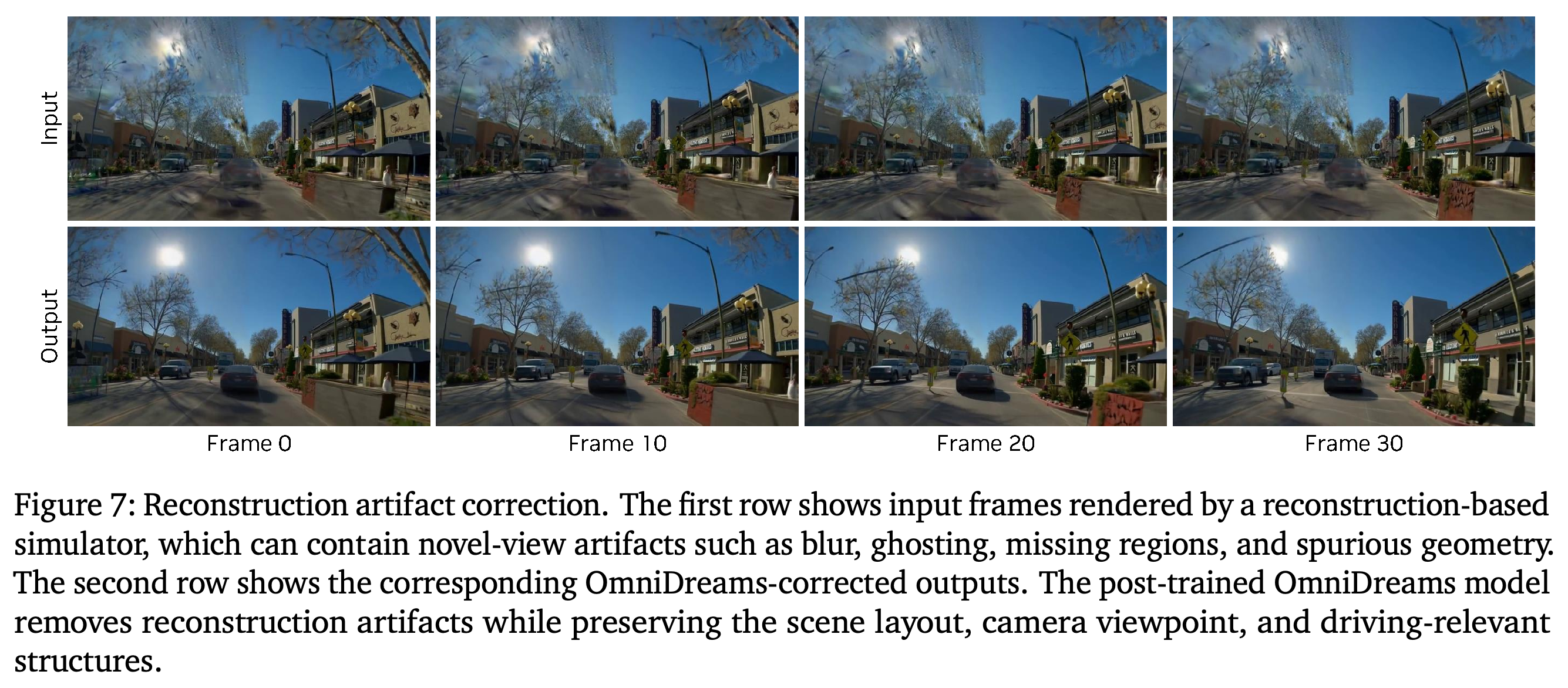
OmniDreams is also post-trained as a diffusion fixer using paired degraded reconstruction renderings and clean target images. Denoising starts from the degraded rendering rather than random Gaussian noise, learning a flow toward cleaner images while targeting preservation of scene layout and viewpoint. At inference, causal history and KV caching condition successive corrections.

• Figure 7 qualitatively compares corrected frames with inputs containing reconstruction artifacts.
• This hybrid use retains reconstruction-based scene grounding, but the section reports no quantitative correction metrics or downstream incident reductions.

Input and corrected outputs at frames 0, 10, 20, and 30 show visibly cleaner renderings with a recognizable road and scene arrangement. The example supports artifact correction qualitatively, but does not quantify geometry preservation or policy benefit.

9. Experiments and Results

The experiments assess appearance and dynamics, long-horizon stability, controllable long-tail scenarios, and closed-loop policy evaluation. Quantitative quality metrics and simulator comparisons are supplemented by qualitative examples of multi-view generation, scenario editing, unusual objects, and reconstruction correction.

9.1. Simulation Quality

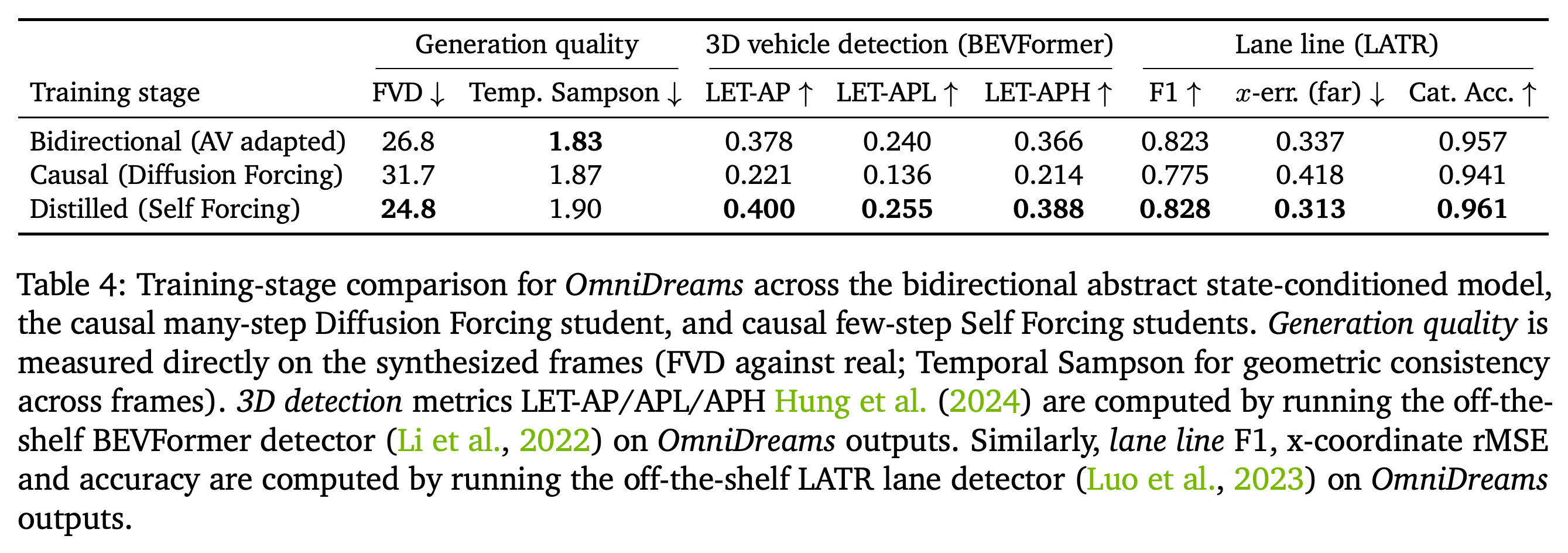
Simulation-quality metrics use 1,000 clips sampled from the 5,000-clip RDS-HQ-1M held-out split. Table 4 shows that Self Forcing improves FVD and all reported vehicle-detection and lane metrics relative to causal Diffusion Forcing, but not Temporal Sampson. Table 5 shows the quality cost of the low-latency LightTAE decoder.

• For bidirectional, causal, and distilled models respectively, FVD is 26.8/31.7/24.8, LET-AP is 0.378/0.221/0.400, and lane F1 is 0.823/0.775/0.828; Temporal Sampson is 1.83/1.87/1.90, with lower being better.
• Replacing the original decoder with LightTAE changes FVD from 24.8 to 45.4, LET-AP from 0.400 to 0.376, lane F1 from 0.828 to 0.813, and Temporal Sampson from 1.90 to 2.02. Section 9.1 calls this LightVAE, but Table 5 and Section 5.1 identify the decoder as LightTAE.
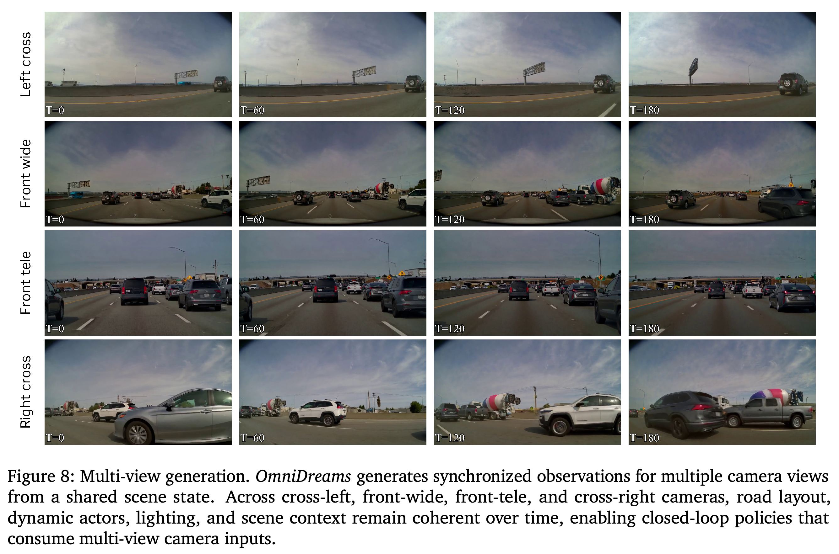
• BEVFormer and LATR provide indirect tests of driving-relevant fidelity. Figure 8 shows qualitative four-camera coherence, but the subsection provides no dedicated numerical cross-view consistency metric.

Four camera rows show an evolving traffic scene at matched times, with shared vehicles and road context across overlapping views. This is qualitative evidence of cross-camera coherence, not a numerical consistency benchmark.

Self Forcing achieves the best FVD, vehicle-detection scores, and lane metrics among the three stages. Temporal Sampson instead favors the bidirectional model at 1.83 over the distilled model at 1.90, so improvement is not uniform across metrics.

LightTAE worsens every displayed quality metric relative to the original decoder, including FVD from 24.8 to 45.4 and lane F1 from 0.828 to 0.813. The fastest deployment therefore does not retain the original-VAE evaluation quality.

9.2. Long Rollouts

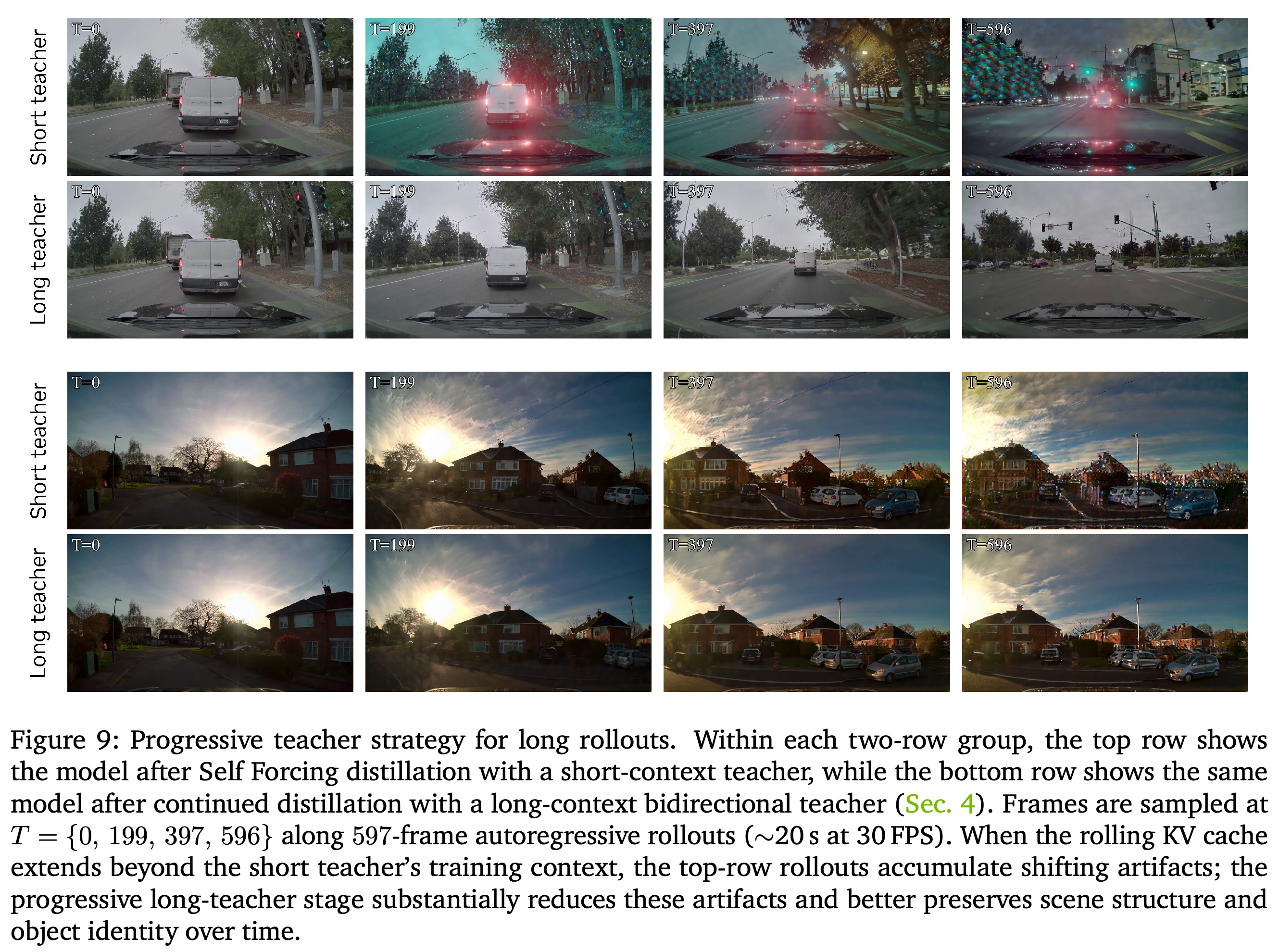
Long-rollout stabilization combines causal KV caching, progressive long-context Self Forcing, bounded temporal attention, and attention-sink tokens from the first RGB frame. Figure 9 compares 597-frame rollouts, approximately 20 s at 30 FPS, using frames T = {0, 199, 397, 596}. Table 6 measures reduced but persistent degradation across four five-second windows against the same real-video front-wide reference distribution.

• Short-context teacher FVD is 109.3, 183.0, 258.3, and 409.2 across successive windows; the progressive teacher yields 95.5, 151.0, 202.5, and 268.4.
• Mean FVD falls from 240.0 to 179.4, while final-minus-first-window Δ falls from 299.9 to 172.9.
• The authors report decent quality over minutes in practice, but the displayed quantitative evidence covers 20-second rollouts.

Matched short- and long-teacher examples at T = {0, 199, 397, 596} show reduced appearance shifts after progressive distillation. The examples span 597 frames, approximately 20 s at 30 FPS, and illustrate better retention of scene structure.

9.3. Long-tail Coverage and Counterfactual Variations

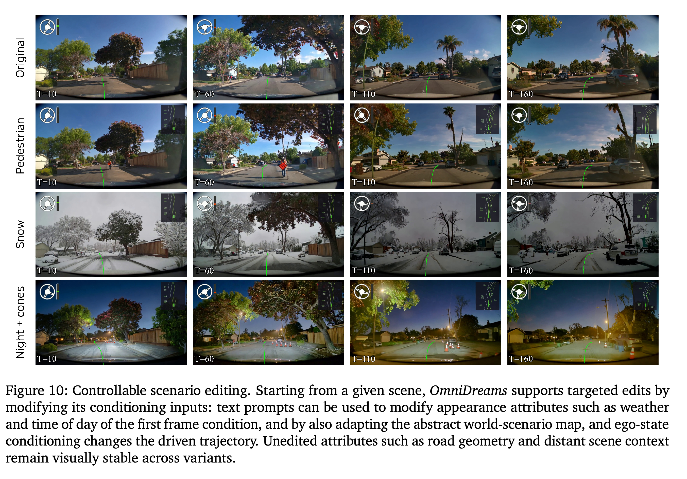
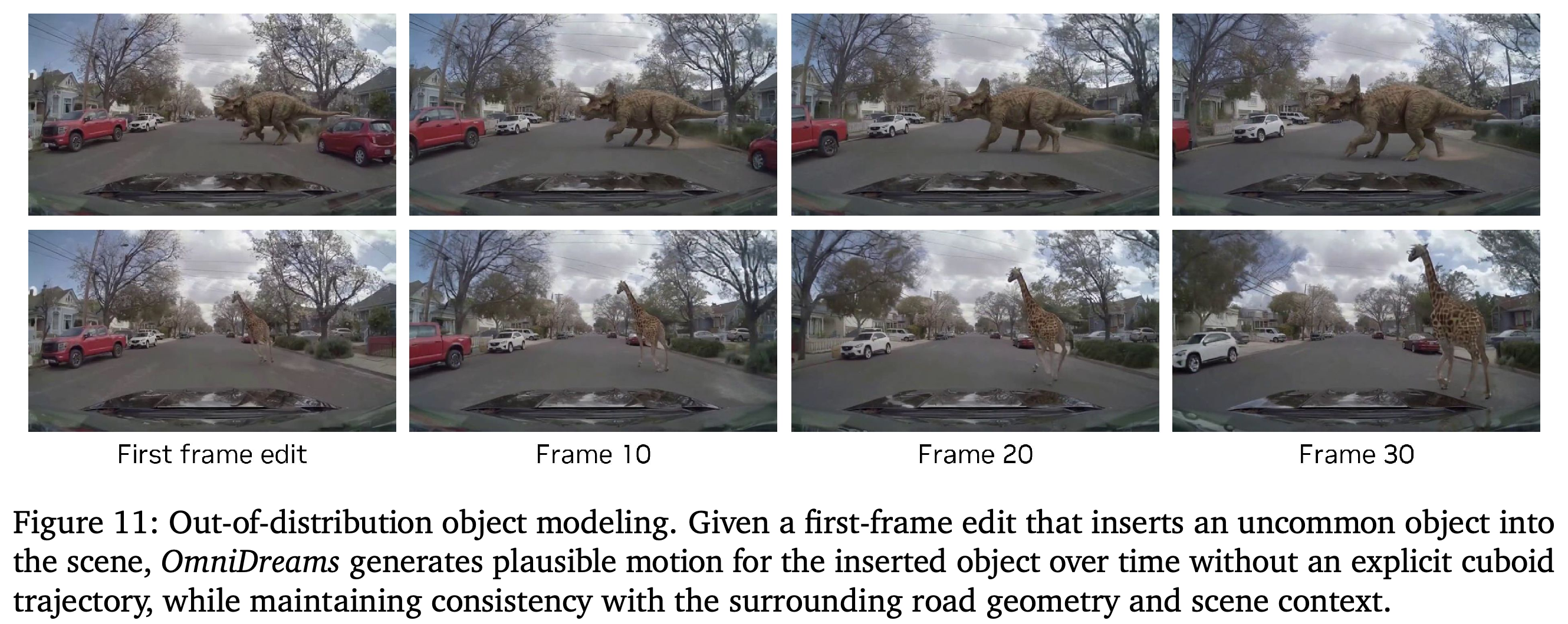
9.3.1. Controllable Scenario Editing uses text, first-frame RGB, and the abstract world-scenario map to vary environmental appearance, scene structure, agents, and ego motion. 9.3.2. Out-of-Distribution Object Modeling introduces a post-trained variant with randomized dropout of dynamic cuboids, allowing unusual objects inserted into the first frame to persist without explicit cuboid trajectories. These demonstrations are qualitative rather than measured long-tail safety coverage.

• Figure 10 compares Original, Pedestrian, Snow, and Night + cones variants while retaining recognizable road geometry and scene context.
• First-frame object insertion can conflict with structured conditioning; dynamic-cuboid dropout teaches greater reliance on visual history and context, while static cuboids such as parked vehicles remain unchanged.
• Figure 11 shows a dinosaur and a giraffe propagated from first-frame edits. Their generated motion is not evidence of explicit simulator control or verified physical behavior.

Original, Pedestrian, Snow, and Night + cones rows show targeted variations on a recognizable seed scene. Persistent road and background context illustrates visual editing, but these examples do not establish invariant geometry or systematic safety-test coverage.

A dinosaur and a giraffe inserted into initial frames remain visible in subsequent generated frames without explicit cuboid trajectories. The examples illustrate the dropout variant’s flexibility, but do not verify physical motion or explicit simulator control of those objects.

9.4. Closed-Loop Evaluation

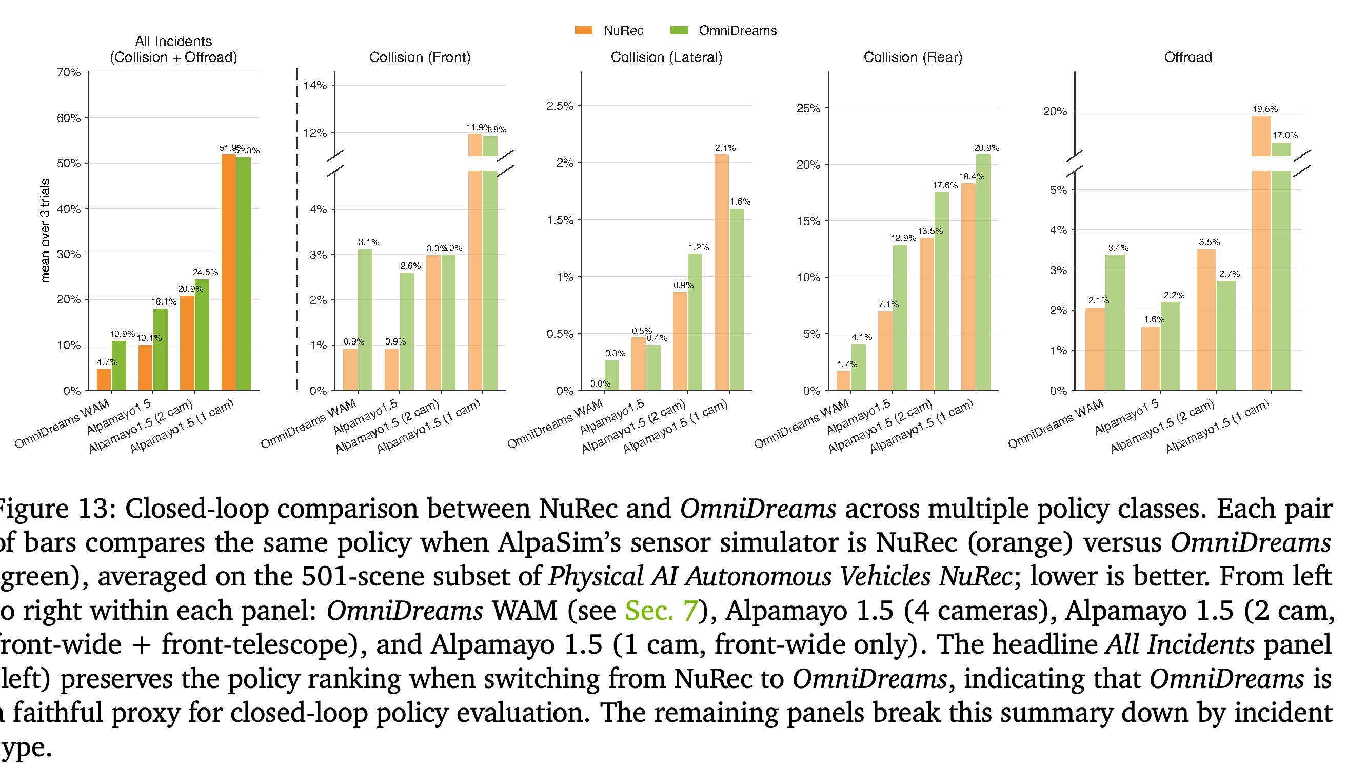
9.4.1. Closed-Loop Comparison to Reconstruction-based NuRec Simulator swaps only the sensor backend while holding AlpaSim, traffic, physics, and per-scene initialization fixed. Evaluation set and metrics. The 501 scenes provide both reconstruction and OmniDreams-compatible conditions and exclude WAM training scenes; each rollout lasts 20 seconds with 533 ms replanning, and incidents count only when the ego is within 4 m of the recorded trajectory. Reported metrics are All Incidents (Collision + Offroad), Collision (Front), Collision (Lateral), Collision (Rear), and Offroad.

• Policies compared. The configurations are OmniDreams WAM and Alpamayo 1.5 with four, two, or one camera; the two-camera configuration uses front-wide and front-telescope, and the one-camera configuration uses front-wide. Results and implications. Three-trial average All Incidents rates for NuRec/OmniDreams are 4.7%/10.9%, 10.1%/18.1%, 20.9%/24.5%, and 51.9%/51.3%, preserving aggregate ranking but not absolute rates.
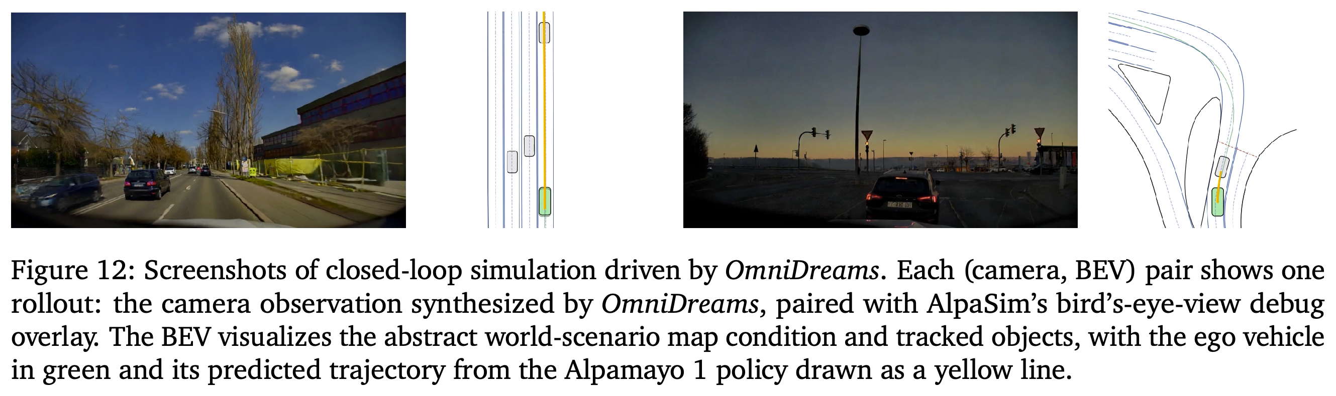
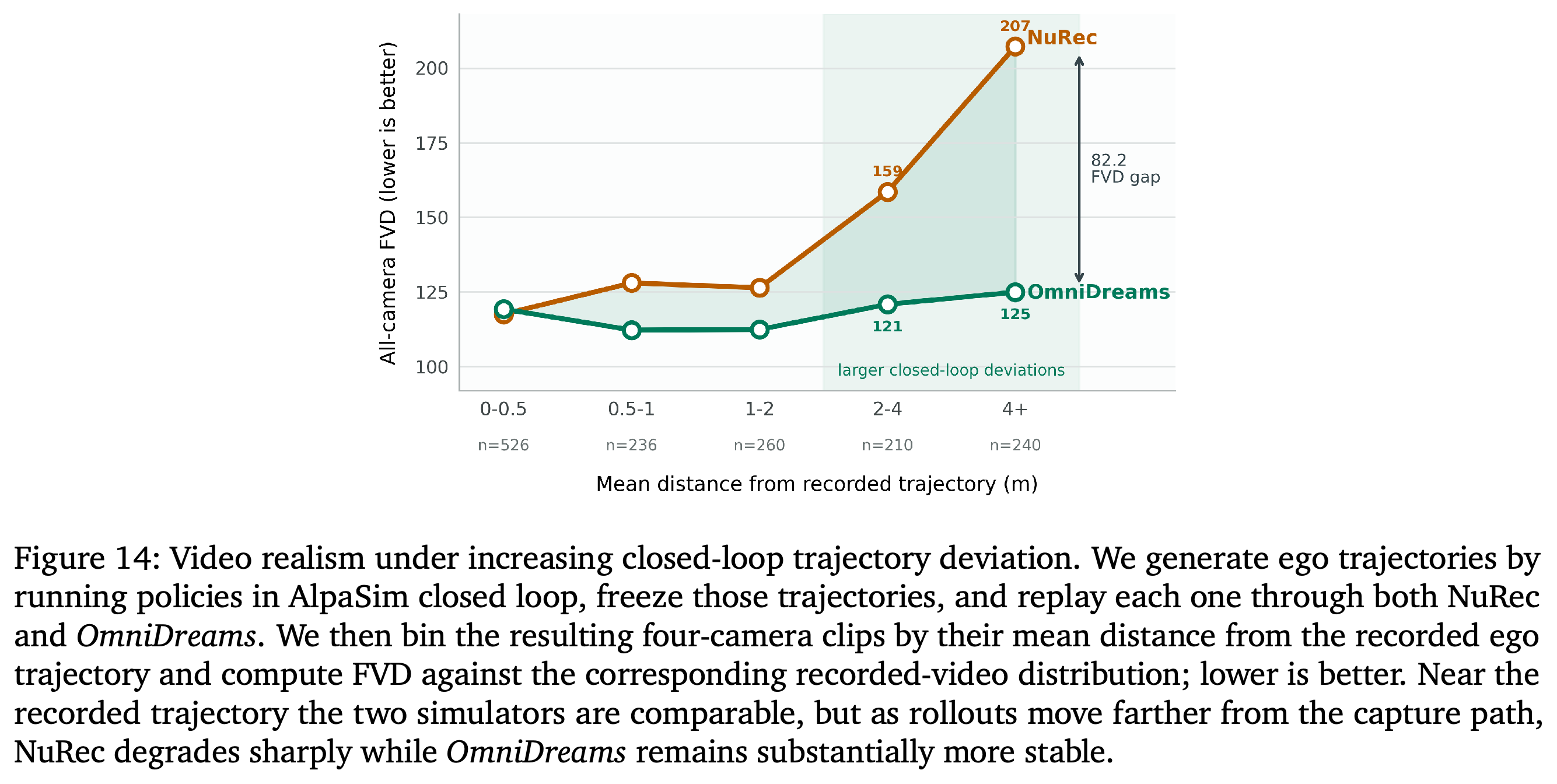
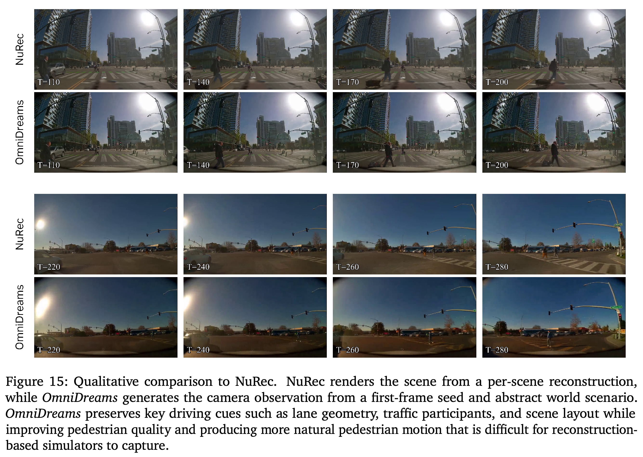
• Visual Realism. Closed-loop trajectories from both backends are frozen and replayed through both renderers. Figure 14 shows comparable FVD near the capture path and a growing advantage for OmniDreams with larger deviations; at 4+ m the plotted values are 207 for NuRec and 125 for OmniDreams, with an annotated 82.2 FVD gap. Figures 12 and 15 provide qualitative rollout and pedestrian examples.
• Controllability and Compute. OmniDreams uses a calibrated first-frame seed and structured world conditions rather than per-scene offline 3DGS reconstruction, but requires substantially more inference compute. Ranking agreement supports comparative evaluation in this tested regime, not calibrated real-world incident probabilities or safety equivalence.

Generated camera observations are paired with AlpaSim BEV overlays showing the ego and its planned trajectory. This connects sensor synthesis to simulator state and policy-driven rollouts rather than standalone offline generation.

Three-trial averages on 501 scenes preserve the All Incidents ordering, with WAM best and one-camera Alpamayo worst under both renderers. Absolute rates differ, including 4.7% versus 10.9% for WAM and 10.1% versus 18.1% for four-camera Alpamayo; the incident-specific panels do not establish identical rankings or rate calibration.

Replaying identical frozen trajectories through both renderers controls requested motion when comparing video distributions. At 2–4 m mean deviation, FVD is 159 for NuRec and 121 for OmniDreams; at 4+ m it is 207 and 125, respectively, supporting better off-capture-path video realism rather than proving geometric accuracy.

Matched crossing sequences show more recognizable pedestrians in OmniDreams outputs than in the corresponding NuRec frames. The comparison illustrates the reported advantage on articulated dynamic content, but provides no dedicated numerical pedestrian-motion metric.

10. Related Work

Related work is organized around sensor-generating world models and infrastructure that connects them to policies. This separates OmniDreams’ causal generation and visual prior from its stateful, distributed, chunk-aware integration into AlpaSim.

10.1. World models for closed-loop AV Simulation

10.1.1. Reconstruction-based World Models discusses NeRF and 3D Gaussian Splatting systems that render captured scenes but have limited coverage of unobserved viewpoints and conditions. 10.1.2. Video models as world simulator reviews Sora, Movie Gen, Wan, Veo 3, Genie, and Cosmos, which OmniDreams specializes for action-conditioned AV simulation. 10.1.3. Generative AV World Models compares driving-video generators with the report’s focus on closed-loop deployment.

• Reconstruction examples include NeuRAD, EmerNeRF, SiMUli, and NuRec; their scene grounding is useful, but extrapolation remains limited by capture coverage.
• Driving-generation examples include DriveGAN, DriveDreamer, GAIA-1/GAIA-2, Vista, MagicDrive, Drive-WM, GenAD, Cosmos-Drive-Dreams, and Waymo World Model. OmniDreams emphasizes streaming caches, few-step inference, and integration with published simulator and policy stacks.
• 10.1.4. Real-time and streaming video diffusion connects the approach to Self Forcing, CausVid, Diffusion Forcing, StreamingT2V, FIFO-Diffusion, StreamingLLM attention sinks, and ring attention; sparse temporal attention and lightweight super-resolution are future extensions.

10.2. Closed-loop AV simulation infrastructure

The infrastructure discussion distinguishes abstract or nonvisual simulators such as Waymax and PufferDrive, artist-asset simulators such as CARLA and MetaDrive, and neural-reconstruction-driven systems such as DriveArena, HUGSIM, WorldEngine, and AlpaSim. The authors propose generative world models as another sensor-realism approach and extend AlpaSim’s microservice architecture for remote distributed rendering and chunk-based state.

11. Conclusion

The report concludes that generative camera simulation can broaden testing conditions beyond reconstruction-only workflows when integrated with a policy and simulation orchestrator. The experiments demonstrate real-time rendering on specified hardware, controllable visual variations, improved off-capture-path FVD, and aggregate policy-ranking agreement in the evaluated setting. The conclusion’s broader connection to safe real-world deployment is not established by these experiments.

Appendix

• B. Glossary consolidates Concepts and acronyms, NVIDIA SIL platform components, Datasets and benchmarks, and Mathematical notation. It defines AV, VLA, WAM, BEV, HD map, VRU, DiT, VAE, AdaLN, RoPE, streaming KV caches, attention sinks, local-window and cross-view attention, context parallelism, Diffusion Forcing, Self Forcing, DMD, and evaluation metrics; platform and dataset entries identify Cosmos, OmniDreams-SV/MV, Cosmos-Drive-Dreams, AlpaSim, Alpamayo, NuRec, SIL-Wheel, GB300, RDS, and RDS-HQ-1M. Latent variables., Noise, conditioning, and parameters., Distributions and operators., and Model functions and distributions. explain latent sequences, Gaussian noise, conditioning, model parameters, expectations, stop-gradient, velocity predictors, and real/fake score networks. Sizes and parallelism axes. distinguishes overloaded symbols: K denotes denoising steps in training but frames per chunk in inference, T denotes sequence length or temporal parallelism, and L denotes loss or rolling-window size; Symbols in tables and prose. explains ↑/↓, →, and ×.

Brief Thoughts

The main contribution is an operational closed-loop integration of causal video generation, with explicit hardware, chunk-size, and policy-timing measurements. Evaluation supports relative policy ranking more directly than absolute incident fidelity: WAM’s All Incidents rate changes from 4.7% under NuRec to 10.9% under OmniDreams. Decoder quality loss, increasing long-rollout FVD, multi-camera compute requirements, and within-chunk trajectory commitment constrain the real-time simulation claim. Progressive teaching reduces temporal degradation with clear numerical support, but does not eliminate it. The preliminary WAM collision result uses a different scene subset and replanning protocol from the renderer comparison and should remain separate. Measured throughput demonstrates feasibility on the specified hardware, not low-cost scalability or real-world safety validation.