Towards a Unified View of Large Language Model Post-Training | Summary

Contents

Summary
1 Introduction
2 A Unified View on Post-Training Algorithms
3 Experiments
- 3.1 Experimental Setup
- 3.2 Main Results
4 Empirical Analysis
5 Conclusion
Appendix
Brief Thoughts

This article explains the key points of Towards a Unified View of Large Language Model Post-Training.

2025-09-04 (arXiv)
Lv, Xingtai, Zuo, Yuxin, Sun, Youbang, Liu, Hongyi, Wei, Yuntian, Chen, Zhekai, Zhu, Xuekai, Zhang, Kaiyan, Wang, Bingning, Ding, Ning, et al.
Tsinghua University, Shanghai AI Laboratory, WeChat AI
Paper
Github

Summary

Post-training, the training performed after pretraining, must combine learning from demonstrations with reward-based learning from a language model’s own generated responses. Hybrid Post-Training (HPT), which selects a training signal using each question’s sampled accuracy, achieves a six-benchmark mathematical reasoning average of 52.7 on Qwen2.5-Math-7B, compared with 49.8 for LUFFY, a baseline combining model-generated responses and external demonstrations, under the paper’s reported evaluation protocol.
The Unified Policy Gradient Estimator (UPGE), a shared expression for parameter-update signals, connects supervised fine-tuning (SFT), learning to reproduce demonstrations, with reinforcement learning (RL), learning from rewards. Its four components are a stabilization mask that suppresses selected updates, a reference policy denominator that reweights samples, an advantage estimate that scores response quality, and a likelihood gradient that maps those signals to model parameters. A policy here is the model’s conditional probability distribution over tokens or responses.
HPT selects SFT when sampled responses perform poorly and RL otherwise, using a binary decision for each question. Results across three pretrained backbones, models used as training starting points, support the tested switching strategy, but incomplete training-data specifications, absent uncertainty estimates, and inconsistent descriptions of the RL implementation limit reproducibility and broader interpretation.

1 Introduction

The introduction identifies complementary failure modes: RL applied directly to a pretrained model can fail when generated responses never receive a useful reward, while SFT can overfit demonstrations and impair generalization to inputs outside the training distribution. Sequential SFT→RL adds a separate training stage, and existing combined objectives leave the relationship between their learning signals insufficiently explained.

Online data means responses generated by the training model; offline data means demonstrations supplied by humans or another model. A rollout is a response sampled from a model policy.
The proposed contribution combines a gradient-level interpretation with question-dependent training selection, allowing the choice of learning signal to change as the model’s performance changes.

2 A Unified View on Post-Training Algorithms

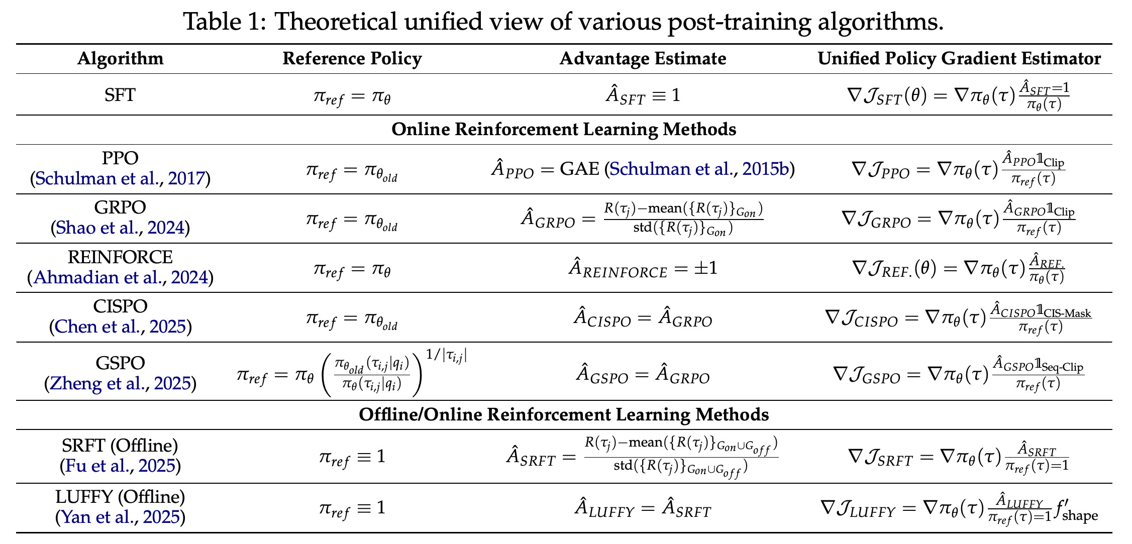
The paper expresses the gradients of SFT and several online and offline RL algorithms in one multiplicative form. Table 1 organizes their differences through denominator, advantage, and masking choices, providing a framework for comparing gradient calculations under stated assumptions. Sharing this form does not give every practical update identical statistical properties.

2.1 Components of the Unified Policy Gradient Estimator

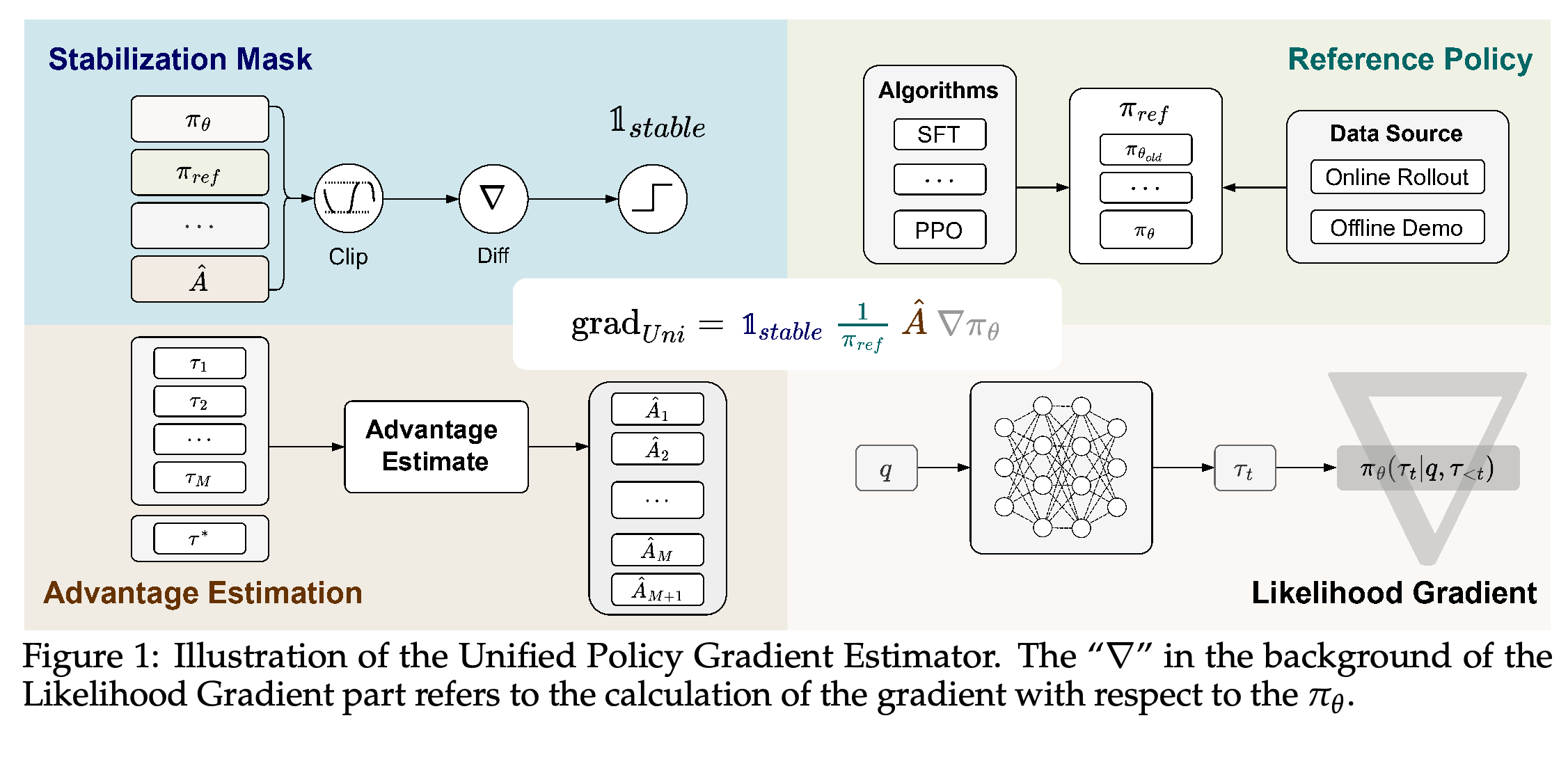
UPGE separates the gradient into four components with different roles: suppressing selected updates, reweighting tokens, assessing response quality, and propagating the learning signal into model parameters. The likelihood gradient is shared across the compared calculations; the other components determine each response’s contribution.

For SFT, the denominator is the current policy probability. For Proximal Policy Optimization (PPO), an RL algorithm that clips policy-probability ratios to constrain updates, it is generally the probability under the policy that generated the responses.
Offline RL methods often set the denominator to 1 because demonstration-generation probabilities are unavailable. The paper’s reference policy denominator is a weighting component and can differ from the rollout policy.
An advantage measures the benefit of an action relative to a baseline; in the language-model setting discussed here, it usually scores an entire response.

The four components of the Unified Policy Gradient Estimator.

Gradient components of representative post-training algorithms.

2.2 Derivation of the Unified Policy Gradient Estimator

The Common Objective maximizes expected reward while penalizing Kullback–Leibler (KL) divergence, a measure of distribution mismatch, from the demonstration policy to the current model. Differentiation produces an RL term sampled from the current policy and an SFT term sampled from the demonstration policy. Importance reweighting, correction for a change in sampling distribution, yields the unified expression under the required support conditions.

Equation 1 is J_μ(θ) = E_{τ∼π_θ(·|q)}[r(τ|q)] − μ KL(π_β(·|q) ∥ π_θ(·|q)), μ ≥ 0, where q is a question, τ is a generated response trajectory, r is its score, and π_β is the demonstration policy.
Equation 4 defines Â_uni(τ,q) = r(τ|q) + μ π_β(τ|q)/π_θ(τ|q). The compact masked estimator is grad_uni = 1_stable (1/π_ref) Â ∇π_θ.
The shared objective permits joint optimization but does not establish that individual SFT and RL gradients always align. Group-relative advantages and clipping introduce the practical estimator differences examined next.

2.3 Gradient Component Analysis

The component analysis examines bias, systematic estimation error, and variance, variability in estimated gradients, introduced by data sources, inverse-probability weights, clipping, and advantage construction. Limited offline datasets cannot satisfy the broad state–action coverage assumptions needed for some RL interpretations. A constant denominator improves numerical stability while introducing bias relative to the importance-weighted interpretation.

Clipping suppresses updates when policy ratios move too far in an unfavorable direction. It can stabilize training while discarding useful signals and introducing bias.
Group Relative Policy Optimization (GRPO), an RL method that compares rewards within a group of sampled responses, centers and normalizes rewards to construct advantages. Other discussed methods use fixed signs or centering without standard-deviation normalization.
The authors motivate weighted combinations as combinations of noisy gradient measurements, conditional on data-distribution assumptions and sufficient samples. They do not derive an optimal weighting rule or quantitatively estimate its bias and variance.

2.4 Hybrid Post-Training with Performance Feedback

HPT generates n responses for each question, checks final-answer correctness using a binary verifier, and defines performance P as the mean verification score. Its instantiated gate selects SFT when P ≤ γ and RL when P > γ, so the mixed loss \(\mathcal L=\alpha\mathcal L_{RL}+\beta\mathcal L_{SFT}\) becomes a binary choice for each question.

With γ = 0, a question receives SFT only when every sampled response is incorrect; any positive sampled accuracy selects RL. The generated responses supply the RL loss, while the demonstration supplies the SFT target.
The broader framework allows feedback functions α = f(P) and β = g(P), but experiments use complementary binary coefficients.
Section 2.4 calls the RL implementation Dr. GRPO, a variant described earlier as using centered rewards without standard-deviation normalization, whereas Section 3.1 calls it GRPO. Equation 11 specifies standard-deviation-normalized advantages, leaving the exact variant ambiguous.

3 Experiments

The experiments test whether performance-dependent switching improves mathematical reasoning across model sizes and families. Comparisons include demonstration-only learning, reward-only learning, sequential training, and methods combining online and offline signals.

3.1 Experimental Setup

The backbones are Qwen2.5-Math-1.5B, Qwen2.5-Math-7B, and LLaMA-3.1-8B. Evaluation covers six mathematical reasoning benchmarks: AIME 2024, AIME 2025, AMC problems from AMC12 2022 and AMC12 2023, MATH-500, Minerva, and OlympiadBench. Qwen2.5-Math-7B additionally receives out-of-distribution evaluation, testing beyond the mathematical training domain, on ARC-c, an open-domain reasoning benchmark, and GPQA-Diamond, a graduate-level question-answering subset.

Evaluation uses an 8,192-token maximum generation length, temperature 0.6, which controls sampling randomness, and top-p 0.95, which restricts sampling to a probability-mass threshold. The main results estimate Pass@1, the probability that one sampled response is correct, using avg@32, accuracy averaged over 32 responses, for AIME 2024, AIME 2025, and AMC, and avg@1 for the other benchmarks.
Training samples 8 responses per question at temperature 1.0, uses AdamW, an optimizer with weight decay, with a constant learning rate of 5 × 10⁻⁶, and runs on 8 × NVIDIA A800 80GB GPUs. The main-experiment gate is γ = 0 for Qwen models and γ = 2/8 for LLaMA.
Baselines include SFT, GRPO, SFT→GRPO, LUFFY, and SRFT, a single-stage supervised and reinforcement fine-tuning method. Some results come from prior papers, and SRFT uses the authors’ implementation because its official code was unavailable.
The PDF does not fully specify the main training datasets, demonstration provenance, batch sizes, or matched compute budgets. It provides code at https://github.com/TsinghuaC3I/Unify-Post-Training.

3.2 Main Results

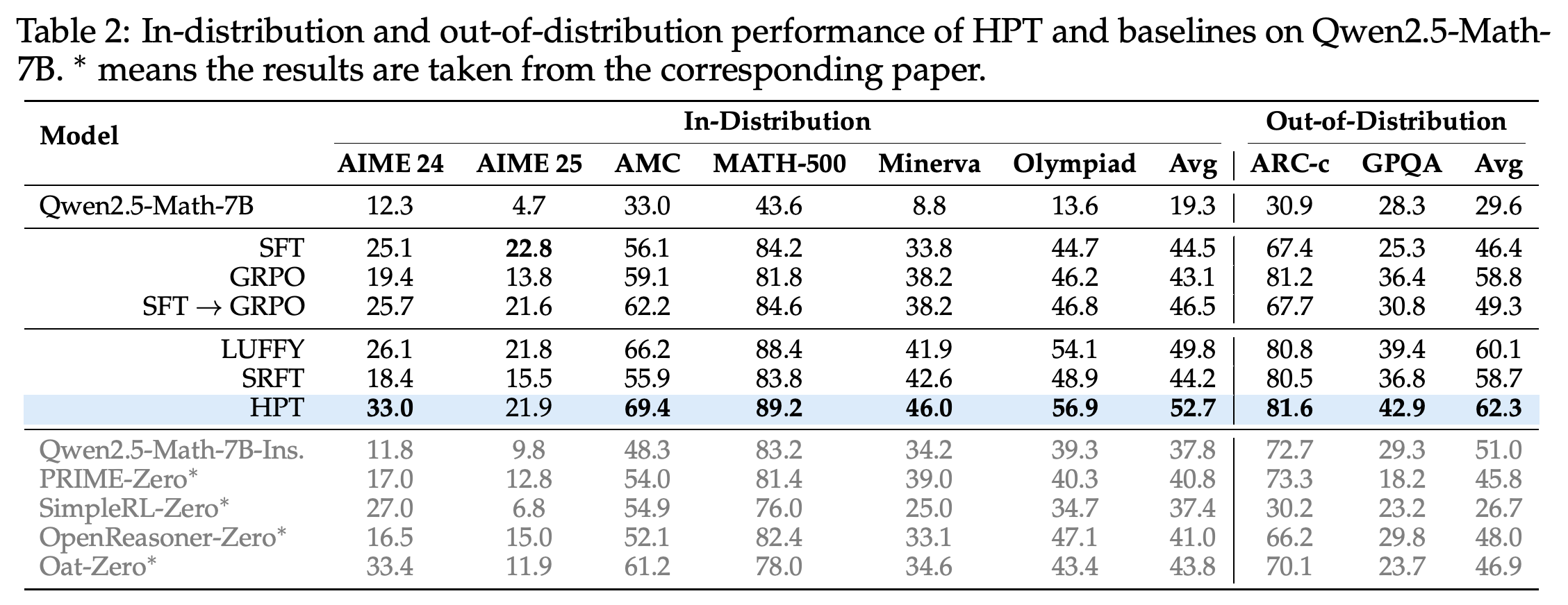
On Qwen2.5-Math-7B, HPT achieves a six-benchmark average of 52.7, versus 44.5 for SFT, 43.1 for GRPO, 46.5 for SFT→GRPO, 49.8 for LUFFY, and 44.2 for SRFT. Its AIME 2024 score is 33.0, exceeding LUFFY’s 26.1 by 6.9 points. Its out-of-distribution average is 62.3 versus LUFFY’s 60.1.

HPT does not lead every individual comparison: SFT scores 22.8 on AIME 2025 versus HPT’s 21.9, and the externally reported Oat-Zero baseline scores 33.4 on AIME 2024.
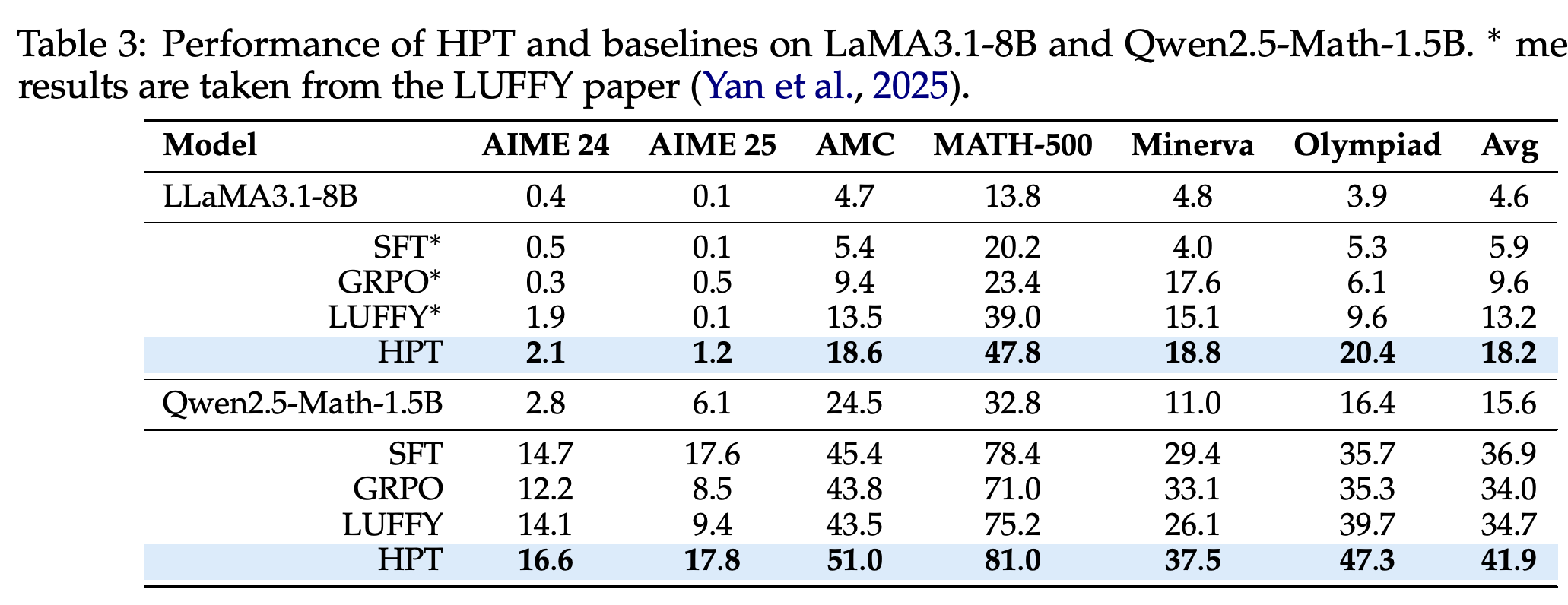
On LLaMA3.1-8B, HPT averages 18.2 versus LUFFY’s 13.2; on Qwen2.5-Math-1.5B, it averages 41.9 versus SFT’s 36.9 and LUFFY’s 34.7. The LLaMA baseline scores are taken from the LUFFY paper.
The tables report point estimates without confidence intervals or variation across training seeds. The claimed computational advantage over sequential training is not accompanied by measured runtime or compute-cost results.

Qwen2.5-Math-7B performance on six mathematical and two out-of-distribution benchmarks.

HPT and baseline performance on LLaMA3.1-8B and Qwen2.5-Math-1.5B.

4 Empirical Analysis

The empirical analysis examines exploration, finding successful responses through sampling, and exploitation, learning from demonstrations. It measures sampled solution coverage, gains and losses on individual problems, training-set learning trajectories, validation accuracy, output diversity, response length, and demonstration use. It then tests alternative offline objectives and switching thresholds.

4.1 Exploration and Exploitation

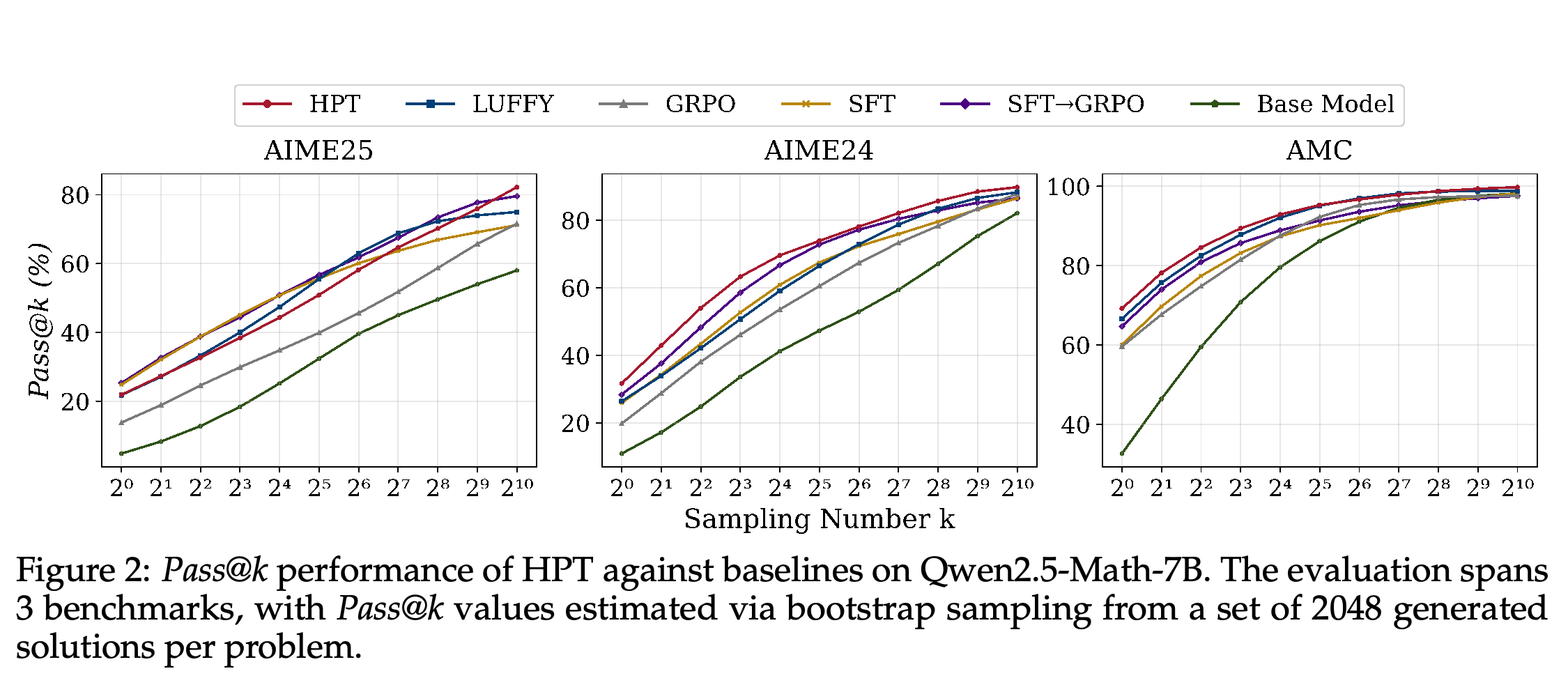
Exploration is measured with Pass@k, the probability that at least one of k sampled responses solves a problem, on Qwen2.5-Math-7B across AIME 2025, AIME 2024, and AMC. Figure 2 estimates values up to k = 1024 by bootstrap sampling, resampling generated solutions to estimate success probabilities, from 2048 solutions per problem. HPT achieves the strongest large-k performance overall in these plots.

The curves support improved sampled solution coverage under this evaluation. The authors suggest that demonstrations introduce useful knowledge and diversity, but the curves do not isolate that causal contribution.
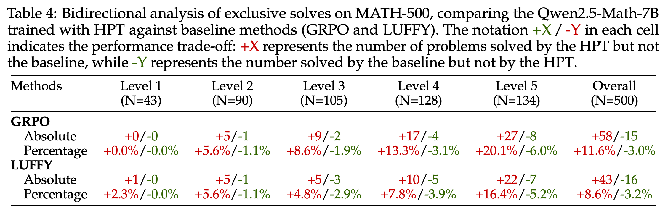
Table 4 compares exclusive MATH-500 solves, problems solved by only one method: HPT solves 58 that GRPO does not, while GRPO solves 15 that HPT does not. Against LUFFY, the corresponding counts are 43 and 16.
At difficulty Level 5, HPT’s exclusive gains and losses are +27/−8 against GRPO and +22/−7 against LUFFY. These counts support gains on difficult problems while showing that some baseline successes are lost.

Pass@k curves on AIME 2025, AIME 2024, and AMC for Qwen2.5-Math-7B.

Exclusive MATH-500 solves gained and lost relative to GRPO and LUFFY.

4.2 Training Visualization

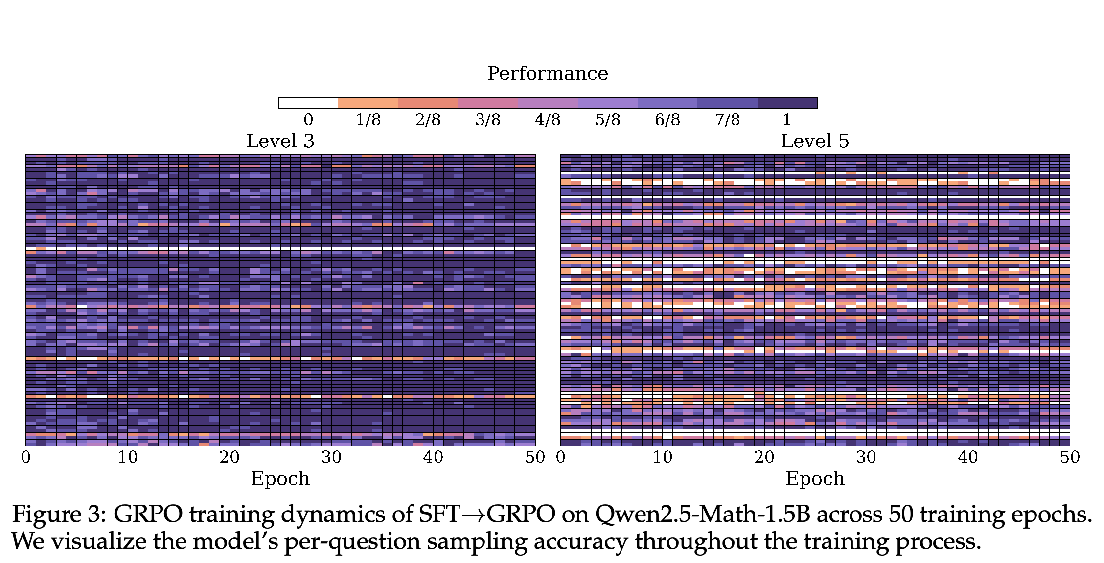
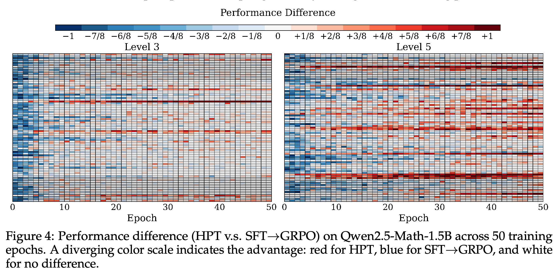
The training visualization uses 255 MATH problems, with 85 each from Levels 3, 4, and 5, and tracks Qwen2.5-Math-1.5B for 50 epochs. The sequential baseline begins its GRPO stage after SFT, while HPT begins from the pretrained backbone without that preceding SFT stage.

Figure 3 contains persistent zero-accuracy rows, especially for Level 5, showing questions for which the sequential baseline’s sampled responses remain incorrect.
Figure 4 compares matched questions and training steps: the sequential baseline initially leads, but HPT gains later, particularly on Level 5. These training-set measurements do not independently establish generalization.
The preceding SFT stage gives the baseline additional training and a different starting point. Section 4.2 also claims that HPT avoids rollouts during SFT updates, but Algorithm 1 requires sampling to determine the gate; the PDF does not explain how that cost is avoided.

Per-question sampling accuracy during 50 epochs of SFT→GRPO training.

Matched-question accuracy differences between HPT and SFT→GRPO.

4.3 Training Dynamics

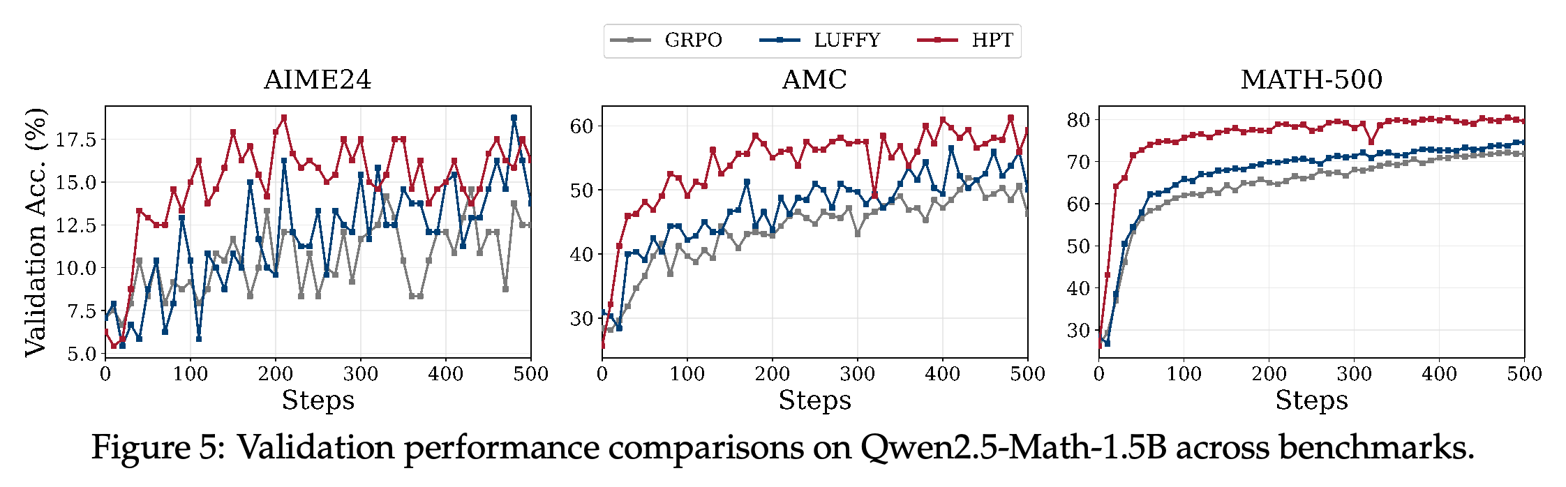
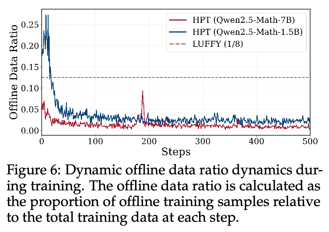
Across 500 training steps, validation curves generally favor HPT over GRPO and LUFFY, while its offline data ratio, the fraction of training samples supplied by demonstrations, falls toward a small nonzero level. Qwen2.5-Math-1.5B initially uses more offline data and transitions later than Qwen2.5-Math-7B.

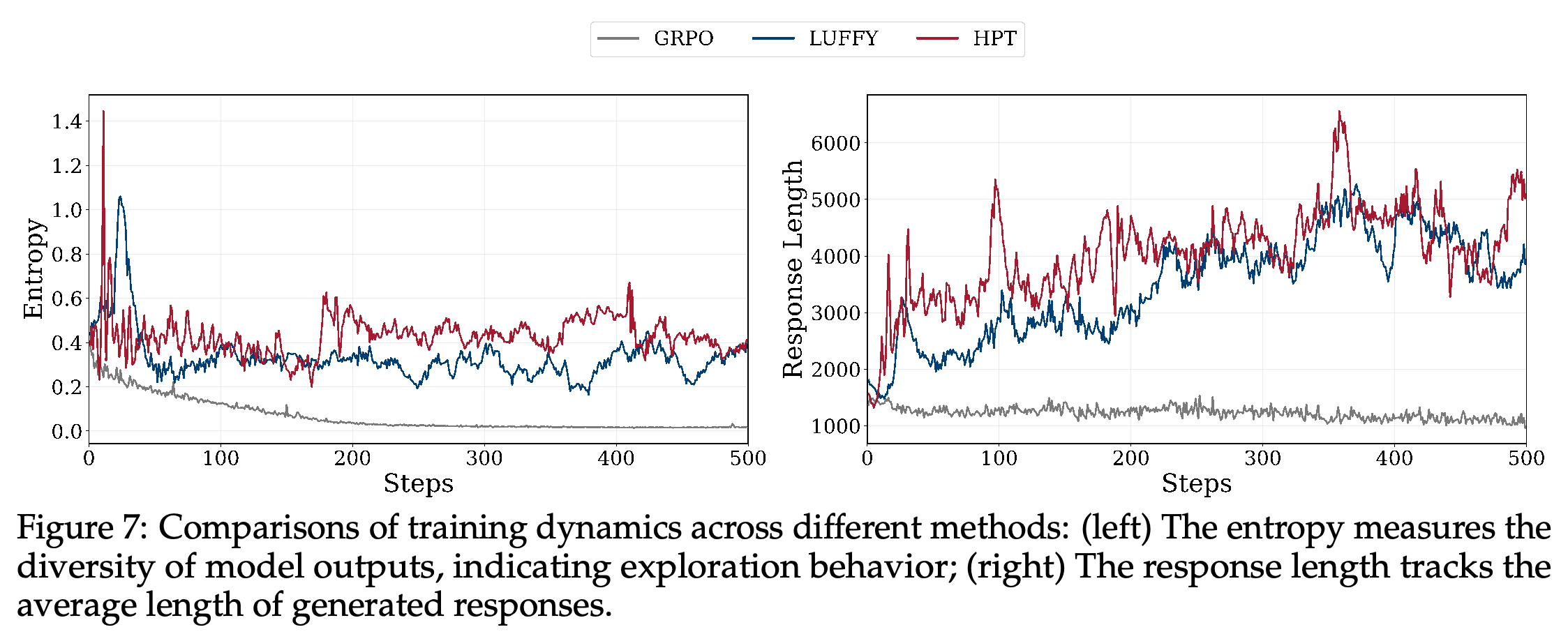
Figure 7 tracks entropy, uncertainty in token probabilities used here as an indicator of output diversity. HPT maintains higher entropy than GRPO, whose curve approaches zero.
HPT’s average response length rises early and remains elevated after the demonstration share decreases. The authors interpret this persistence as retention of learned reasoning patterns, but length alone does not establish their content or correctness.
Figure 6 defines the offline ratio in terms of samples, although the surrounding prose also discusses prompts. The plotted ratio should therefore not be treated directly as the fraction of questions assigned to SFT.

Validation accuracy over training steps on Qwen2.5-Math-1.5B.

Offline training sample ratios for HPT and the fixed LUFFY reference.

Token entropy and average generated response length during training.

4.4 Impact of Off-policy RL

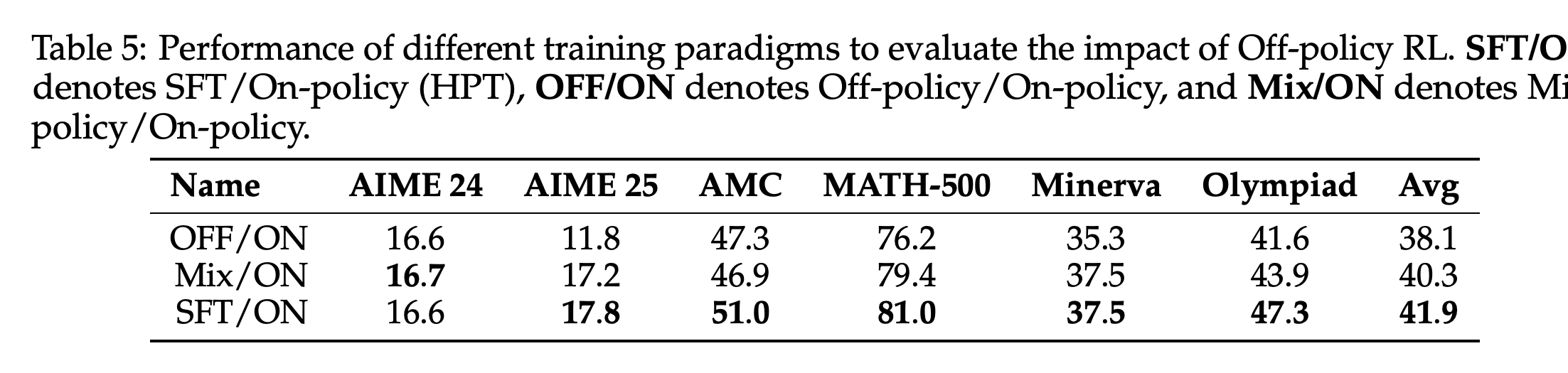
The offline-data ablation compares SFT/ON, HPT’s alternation between SFT and on-policy RL using current-model responses; OFF/ON, alternation between off-policy RL using external demonstrations and on-policy RL; and Mix/ON, a combined offline objective switched with on-policy RL. Their six-benchmark averages are 41.9, 38.1, and 40.3, respectively.

For Mix/ON, the selected SFT/OFF weighting ratio is 1/10, implemented with coefficients 0.1 and 1.0. The off-policy implementation follows LUFFY, and the paper states that the experimental settings are shared.
SFT is the better tested offline component by average score in this setting. The comparison does not establish that off-policy RL is unnecessary across other data distributions, models, or implementations.

Performance of alternative offline and online training combinations.

4.5 Gate Threshold Ablation

On Qwen2.5-Math-1.5B, thresholds γ = 0, γ = 1/8, and γ = 2/8 yield six-benchmark averages of 41.9, 38.7, and 39.0, respectively. Higher thresholds increase demonstration use but do not improve the overall average. γ = 1/8 nevertheless gives the highest AIME 2024 score, 18.1.

The formal gate uses RL only when P > γ. With 8 responses per question, thresholds 0, 1/8, and 2/8 therefore require at least 1, 2, and 3 correct responses, respectively; Section 4.5’s prose describes the latter boundaries inconsistently and refers to questions where responses are meant.
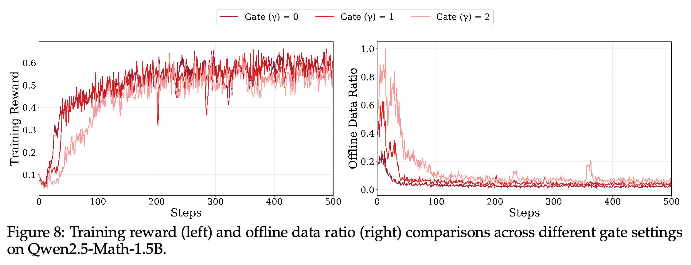
Figure 8 shows that higher gates increase early offline-data use and can slow initial reward improvement. This ablation identifies the best tested threshold for Qwen2.5-Math-1.5B; the main LLaMA experiments use 2/8 without a corresponding threshold comparison.

Training reward and offline data ratio under three switching thresholds.

Qwen2.5-Math-1.5B benchmark performance under different switching thresholds.

5 Conclusion

The conclusion combines a shared gradient formulation with an algorithm that selects demonstration-based or reward-based learning using current performance. The results support HPT’s effectiveness for the tested reasoning backbones and benchmarks. The theoretical interpretation remains conditional on sampling assumptions and the differences among practical gradient estimators.

Appendix

A Gradient Derivation for Classical Algorithms supplies the concrete gradient calculations underlying the comparison. A.1 Gradient of SFT differentiates token-level cross-entropy, the negative log-probability of demonstration tokens, to obtain inverse-current-probability weighting and interprets SFT as behavioral cloning, imitation of demonstrated responses. A.2 Gradient of Online RL: PPO, GRPO and Beyond derives the clipped policy-ratio gradient and GRPO’s group-normalized rewards while omitting KL and entropy regularization terms; A.3 Gradient of Offline RL derives SRFT’s constant-denominator, unclipped update under an offline coverage assumption.
B Additional Theoretical Details for Section 2.2 provides the derivation’s mathematical conditions. B.1 Deriving Equation 2 from Equation 1 uses score-function identities, which differentiate policy expectations through log-probability gradients, and measure-change identities, including the requirement that the sampling density be positive wherever the current policy is positive. B.2 Extension: Adding a Trust-Region Regularizer adds a penalty discouraging large policy changes and modifies the advantage with a log-policy-ratio term; B.3 PPO Clipping and the Stabilization Mask shows how the clipped surrogate objective’s piecewise derivative suppresses updates beyond the trusted range in an unfavorable direction.

Brief Thoughts

HPT provides a simple response to a concrete training failure: when a question produces no successful sampled answers under the Qwen default gate, a demonstration supplies a learning signal. The three-backbone results, exclusive-solve analysis, and threshold ablation support this design. They do not establish that the binary gate optimally combines biased gradient estimates. Reproduction requires resolving the GRPO versus Dr. GRPO description, specifying the training-data pipeline, and using the formal gate equation to interpret threshold boundaries. Higher entropy, longer responses, and large-k success provide complementary behavioral evidence, but they do not directly establish retention of particular reasoning mechanisms. A common regularized objective also does not guarantee alignment of every constituent gradient.