LiveTradeBench: Seeking Real-World Alpha with Large Language Models | Summary

This article explains the key points of LiveTradeBench: Seeking Real-World Alpha with Large Language Models.

• 2025-11-05 (arXiv)
• Yu, Haofei, Li, Fenghai, You, Jiaxuan.
• University of Illinois, Urbana-Champaign
• Paper
• Github
• Project Page

Read this article in Korean

Summary

• LiveTradeBench tests whether large language models (LLMs) can repeatedly allocate a portfolio, a collection of asset holdings, as market prices and information change independently of their actions. Across 21 models evaluated in the same agent framework over 50 trading days, higher LMArena scores, a human-preference measure of general model performance, did not imply better trading returns in either U.S. stocks or Polymarket, a market for contracts on event outcomes. The reported Spearman rank correlations, which compare model rankings, were 0.054 for stocks and −0.38 for Polymarket.
• The benchmark supplies live prices, news, and recent portfolio history, then asks models to allocate capital across 15 U.S. equities or ten binary prediction markets, which offer YES and NO outcomes, with cash available in both settings. GPT-4.1 achieved the highest stock cumulative return, the percentage change in portfolio value, at 6.25%, but returned −33.69% in Polymarket; Claude-Sonnet-3.7 led Polymarket with 20.54%. Model rankings therefore differed substantially between the two markets during the tested period.
• Using older portfolio decisions generally reduced returns at longer delays, especially in Polymarket, supporting a benefit from timely updates in this evaluation. The environment simulates portfolio changes using live data and excludes transaction fees, bid–ask spreads, the difference between buying and selling quotes, and liquidity constraints, limits on trading available quantities at quoted prices. These results do not establish returns after execution costs or persistent alpha, excess return relative to a comparison investment.

1. Introduction

The introduction argues that fixed-input evaluations miss adaptation to delayed, noisy feedback in an independently evolving environment. LiveTradeBench combines live information, allocation across multiple assets, and evaluation in U.S. stocks and Polymarket to test sequential decision-making under uncertainty.

• Historical backtesting, evaluation on past market data, can expose models to information already present in training data. Live evaluation reduces this risk by observing newly evolving markets.
• The authors distinguish trading from the controllable web and computer environments discussed in the paper: an allocation changes the agent’s holdings while the external market continues evolving.
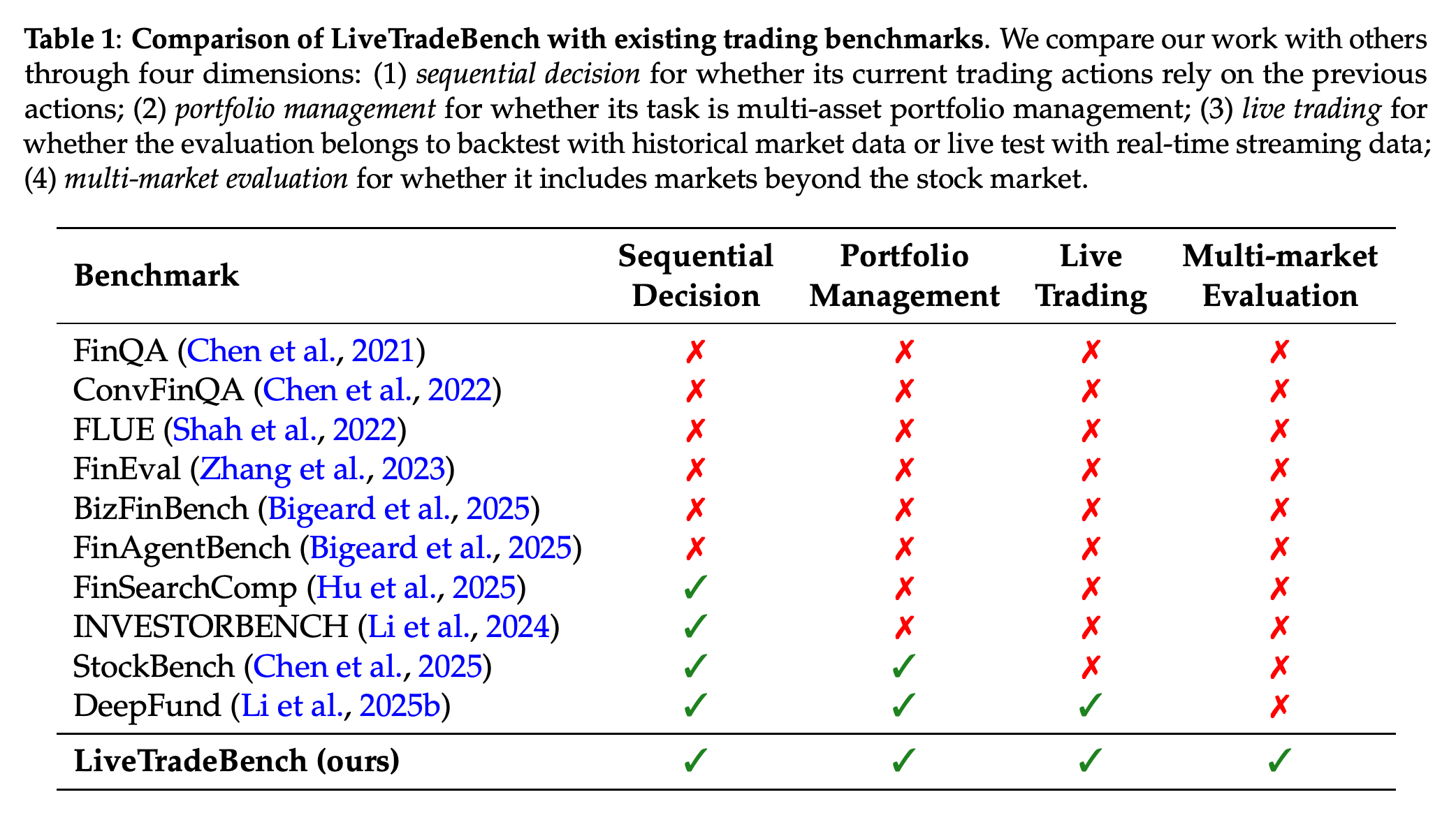
• Table 1 compares sequential decisions, portfolio management, live trading data, and evaluation beyond stocks. These dimensions describe benchmark design rather than trading profitability.

LiveTradeBench satisfies all four listed design dimensions. DeepFund already satisfies sequential decisions, portfolio management, and live trading, so evaluation across multiple market types distinguishes LiveTradeBench in this comparison; the table does not compare returns.

2. Related Work

The related work organizes trading evaluation into historical backtesting, synthetic market simulation, and live evaluation. It compares discrete single-asset actions, expected excess-return predictions, and event-probability estimates, motivating a common action representation based on portfolio allocation.

• Backtesting raises information-contamination and generalization concerns; synthetic markets support behavioral analysis but may differ from actual market dynamics.
• Portfolio weights, the fractions of capital assigned to assets, connect predictions to holdings while representing risk trade-offs and relationships across assets.
• Existing frameworks include reinforcement learning, training from feedback on actions, and collaboration among multiple agents. This study uses a common ReAct framework, which combines explicit reasoning with actions, together with tools and memory of recent observations.

3. Building Live Trading Environment for Portfolio Management

The environment separates externally supplied market evolution from simulated portfolio adjustment. Its design defines the portfolio task, selects two markets, and specifies the observations and allocation actions shared across both settings.

3.1. Definition of Portfolio Management

Portfolio management is formulated as a partially observable Markov decision process (POMDP), a sequential decision model in which the true market state is not fully observed. The observation \(\mathbf{o}_t=(\mathbf{q}_t,\mathbf{p}_t,c_t)\) contains holdings, prices, and contextual information; portfolio value is v_t = q_t^T p_t, and the action specifies target allocation weights summing to one.

• Equation (2) values existing holdings at the next prices, then converts the target weights into new holdings through element-wise division by those prices. Rebalancing preserves portfolio value in this cost-free formulation.
• The trade vector \(\Delta\mathbf{q}_t=\mathbf{q}_{t+1}-\mathbf{q}_t\) maps positive changes to BUY, negative changes to SELL, and zero changes to HOLD.
• The authors assume individual simulated trades have negligible effects on external prices because the selected assets are sufficiently liquid. Low-level order execution is outside the model.

3.2. Market Selection

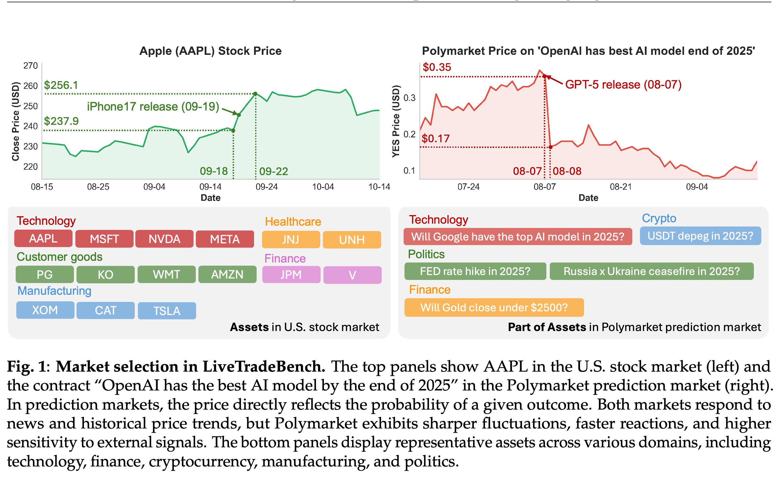
The selected markets test allocation under different information flows: U.S. equities provide sector relationships and exposure to company and macroeconomic developments, while Polymarket contracts respond to information about specific events. The paper hypothesizes that prediction markets react with different latency and magnitude from stocks; this motivates the comparison without establishing a universal property of either market.

• The 15 stock tickers are AAPL, MSFT, NVDA, META, JPM, V, XOM, CAT, TSLA, PG, KO, AMZN, WMT, JNJ, and UNH. Cash has a constant unit price and zero return.
• Ten active binary Polymarket markets cover politics, cryptocurrency, technology, and finance, including questions about a Federal Reserve rate hike, Tether insolvency, a U.S. recession, and “USDT depeg in 2025?”, an event concerning loss of a currency peg.
• Figure 1 illustrates the comparison using AAPL prices around the iPhone17 release and an OpenAI-related prediction contract around the GPT-5 release.

The examples associate AAPL’s movement from $237.9 to $256.1 with the iPhone17 release and a prediction contract’s movement from $0.35 to $0.17 with the GPT-5 release. They illustrate different event-related price patterns in the selected markets without establishing a general causal response rule.

3.3. Observation Space

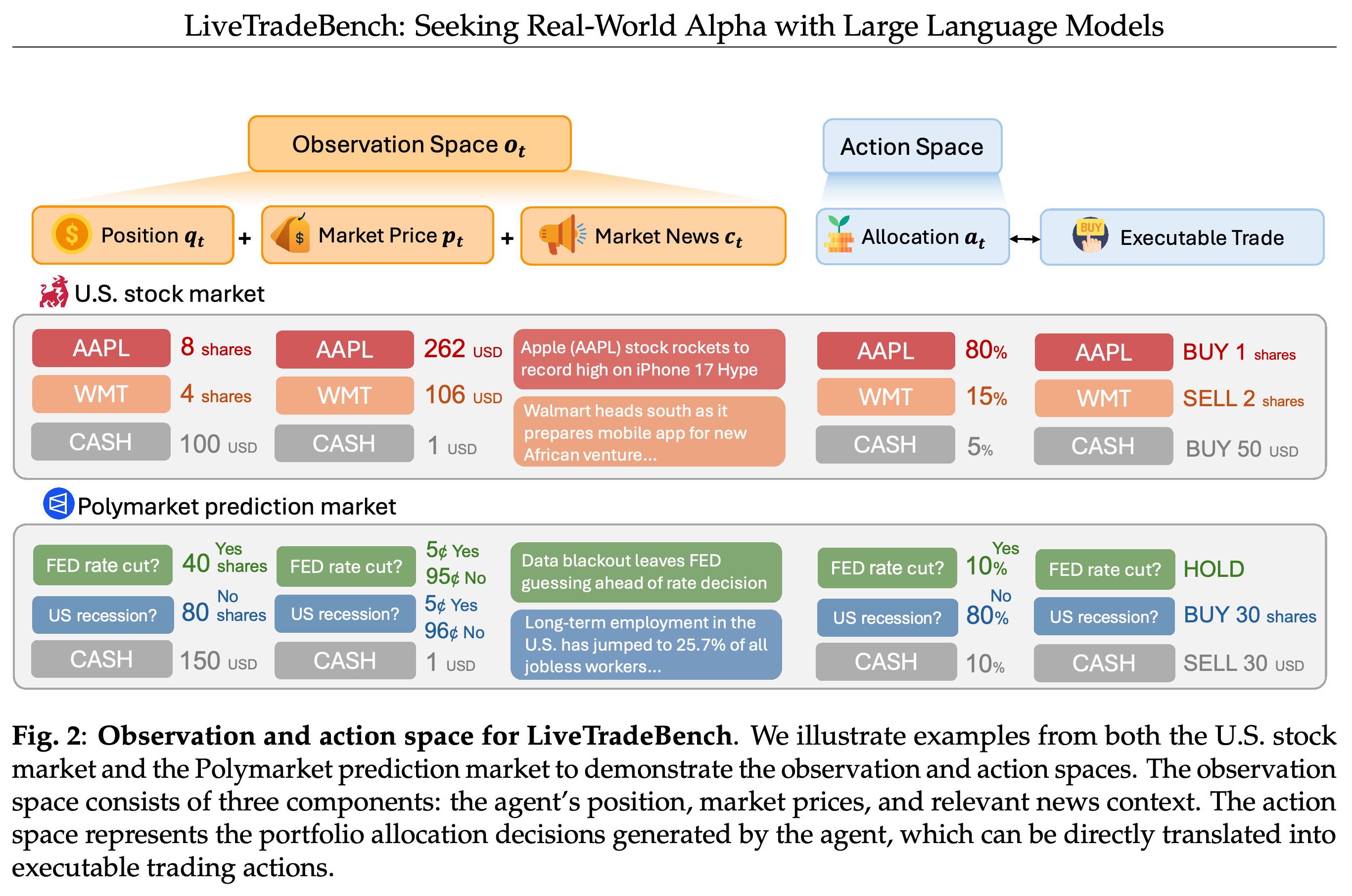
Each observation combines current asset holdings, timestamped market prices, and textual news context. Holdings are continuous and non-negative, so the default setting permits fractional positions but excludes short selling, positions that profit from falling asset prices.

• Stock observations include closing prices for the 15 selected equities; prediction-market observations include prices for ten Polymarket markets.
• Google News queries use asset and topic keywords. News summaries enter the prompt to supply company events, policy expectations, and other contextual signals.
• Figure 2 shows how these inputs lead to allocation weights and corresponding buy, sell, or hold operations in both markets.

Both examples use holdings, prices, and news as observations, then represent decisions as portfolio percentages that map to trades. The diagram explains the common interface across equities and event outcomes; its numerical examples illustrate the interface rather than evaluated model results.

3.4. Action Space

Actions lie on a probability simplex, non-negative weights whose sum is one: \(\sum_i a_t^{(i)}=1\) and a_t^(i) ≥ 0. Stock weights specify capital allocated to each equity, while every binary prediction market has separate YES and NO outcome assets.

• For k prediction markets, the paper describes 2k outcome components; the implemented prompts also allow CASH and require at most one non-zero outcome allocation per question.
• Net event exposure is e_t^(k) = a_{t,YES}^(k) − a_{t,NO}^(k), with positive exposure favoring YES.
• This representation focuses evaluation on portfolio rebalancing, adjustment toward target asset weights, while abstracting away order execution.

4. Designing LLM-based Agents for Portfolio Management

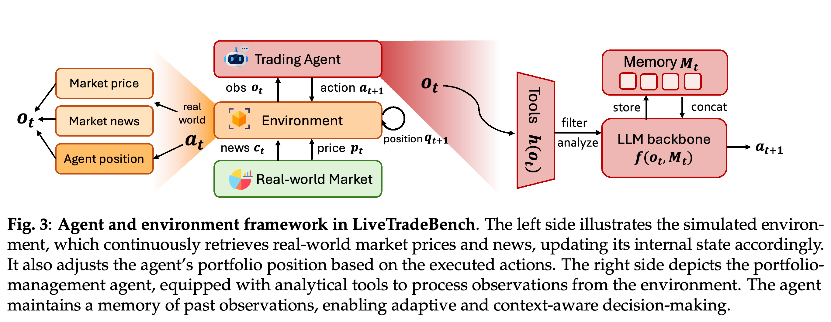
The agent produces allocations through \(\mathbf{a}_t=f_{\theta}(\mathbf{o}_t,\mathbf{M}_t)\), conditioning on the current observation and a memory of previous observations. Its three components are tools for obtaining and processing information, memory for recent temporal context, and explicit reasoning before an allocation is returned.

• Tools transform raw observations into structured quantitative features and relevant textual information, represented as õ_t = h(o_t).
• Memory is M_t = {o_τ | t − Δ ≤ τ < t}, where Δ is the retained history horizon. Past observations are concatenated to provide context about prices, allocations, and portfolio outcomes.
• The ReAct-style framework generates explanations that can be inspected alongside actions. The study evaluates existing model backbones, the underlying LLMs that produce decisions, rather than introducing a training algorithm.

Real-world prices and news enter a simulated environment that updates portfolio positions. The agent processes observations with tools and retained history before producing allocations, showing how live external data and simulated portfolio execution coexist in the benchmark.

5. Evaluating LLM-based Agents under Live Test

The live evaluation covers August 18, 2025, to October 24, 2025, reported as 50 trading days, with 21 unique LLM backbones. The analyses compare financial outcomes, relationships with general model scores, sensitivity to delayed decisions, and information mentioned in allocation explanations.

5.1. Backbone LLMs for Evaluation

All models use the same agent framework to convert observations into prompts and parse outputs into portfolio weights. The evaluated pool spans Claude, Grok, Qwen, Llama, GPT, Gemini, Kimi, and DeepSeek variants, with differences in model size and reasoning style.

• Table 2 includes four Claude models, two Grok models, three Qwen models, three Llama models, four GPT models, two Gemini models, Kimi-K2-Instruct, DeepSeek-V3.1, and DeepSeek-R1.
• The shared framework reduces differences in prompt formatting and execution. It does not isolate intrinsic reasoning ability as the sole cause of outcome differences.
• Section 5.1 initially states six representative families, but Table S1 lists eight family or provider rows. The concrete 21-model inventory gives the more precise description of the evaluated pool.

5.2. Trading Metrics for Evaluation

The evaluation reports five metrics: cumulative return (CR), Sharpe ratio (SR), average return above a risk-free comparison divided by return volatility, maximum drawdown (MDD), the largest decline from an earlier portfolio peak, win rate (WR), the fraction of profitable steps, and volatility, variability in returns. Higher CR, SR, and WR are preferred, while lower MDD and volatility are preferred.

• The definitions include \(CR=\frac{v_T-v_0}{v_0}\) and \(SR=\frac{\bar r-r_f}{\sigma}\), where r_f is the risk-free return and σ is return volatility.
• The stock risk-free comparison is a short-term Treasury yield; the Polymarket comparison is zero because the paper assumes no yield on its stablecoin-denominated assets, assets denominated in a token intended to maintain a stable currency value.
• The introductory paragraph mentions four metrics, but the detailed definitions and Table 2 also include WR. The supplied definitions do not fully specify the scaling or annualization behind the reported SR and volatility values.

5.3. Evaluation Results

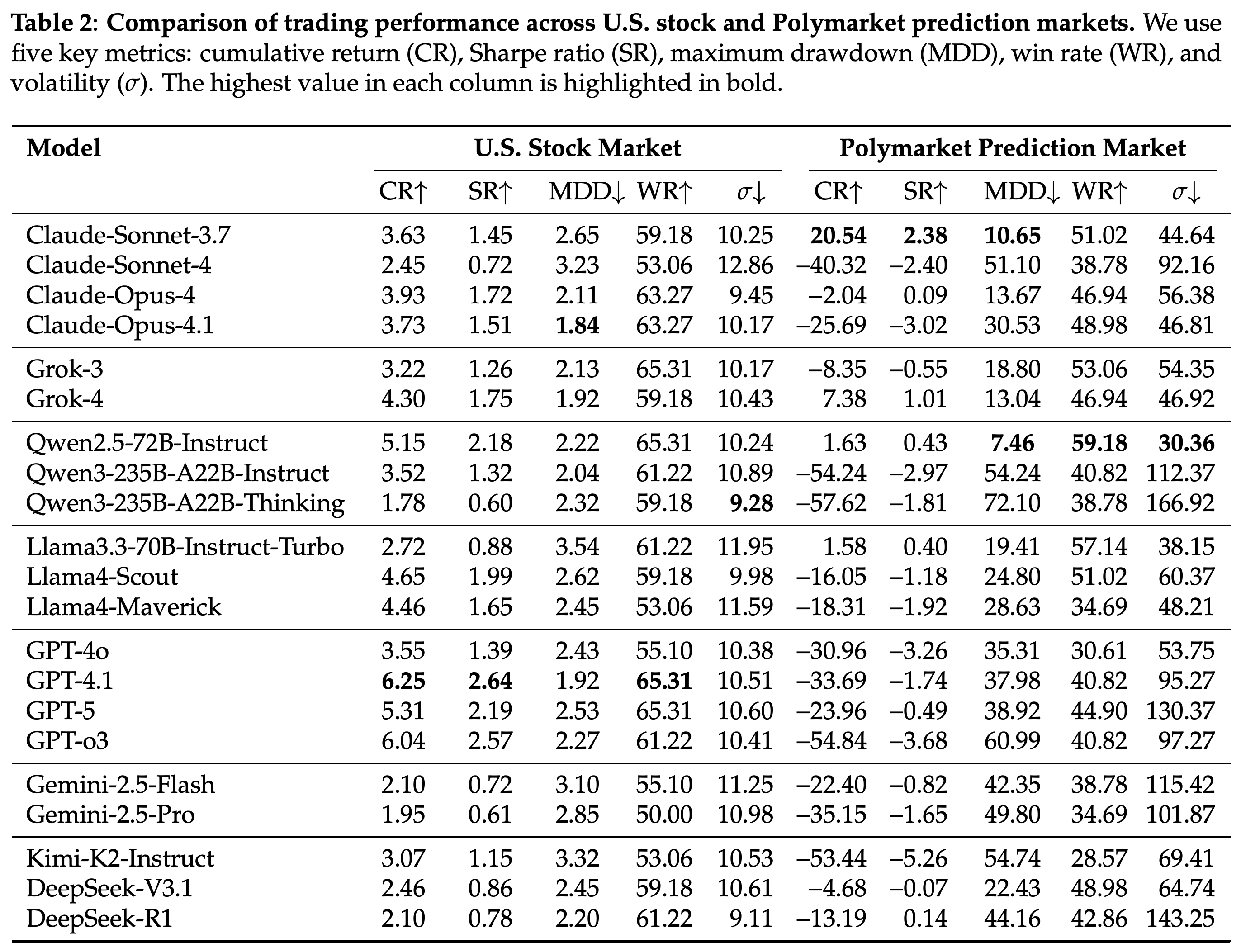
Table 2 shows that the best model depends on the market: GPT-4.1 leads stocks with CR 6.25% and SR 2.64, while Claude-Sonnet-3.7 leads Polymarket with CR 20.54% and SR 2.38. The paper reports a near-zero relationship between the two markets’ Sharpe ratios and Spearman correlations between LMArena scores and cumulative returns of 0.054 for stocks and −0.38 for Polymarket.

• GPT-4.1 returns −33.69% in Polymarket, and GPT-o3 returns 6.04% in stocks but −54.84% in Polymarket. Grok-4 and Qwen2.5-72B-Instruct have positive cumulative returns in both markets.
• Qwen2.5-72B-Instruct has Polymarket MDD 7.46%, WR 59.18%, and reported volatility 30.36, combining modest positive return with the lowest listed prediction-market drawdown and volatility.
• The authors describe distinct asset and cash preferences: GPT-4o concentrates on AAPL, MSFT, and NVDA; GPT-5 diversifies more broadly; Llama4-Scout holds cash above 20%, while GPT-5 keeps it below 10% except under extremely high-risk conditions.
• The reasoning-model discussion requires qualification: DeepSeek-R1 and Qwen3-235B-A22B-Thinking have Polymarket volatility 143.25 and 166.92, respectively, but GPT-o3 is 97.27. The prose’s claim of volatility above 140 does not apply to all three named models, and GPT-o3 has the second-highest stock return.
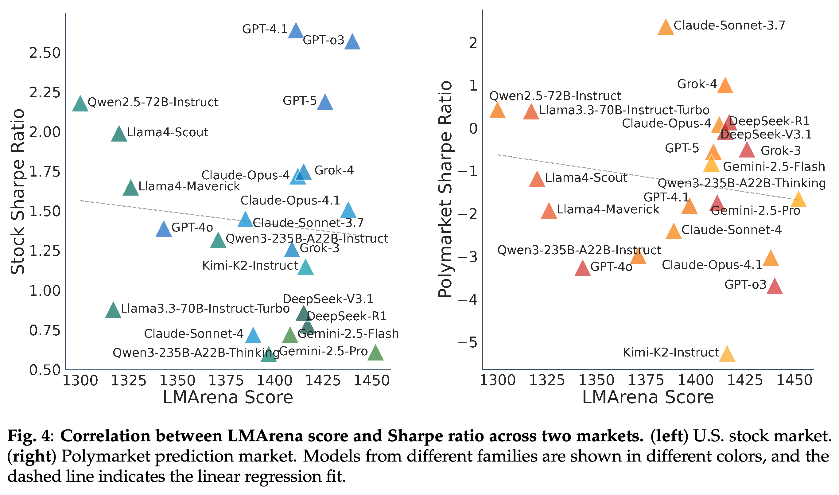
• Figure 4 plots SR against LMArena scores, whereas the numerical Spearman correlations in the text concern cumulative returns. The plots and coefficients describe different outcome measures.

GPT-4.1 leads stocks with 6.25% cumulative return and Sharpe ratio 2.64, while Claude-Sonnet-3.7 leads Polymarket with 20.54% and 2.38. GPT-4.1’s −33.69% Polymarket return demonstrates the change in ranking across markets, and Qwen2.5-72B-Instruct combines positive Polymarket return with the smallest listed drawdown and volatility.

The scatterplots show substantial variation in Sharpe ratios among models with similar LMArena scores, with slightly downward fitted lines. They show no simple positive relationship in this sample, but plot Sharpe ratios rather than the cumulative returns used for the text’s reported Spearman coefficients.

5.4. Analysis and Discussion

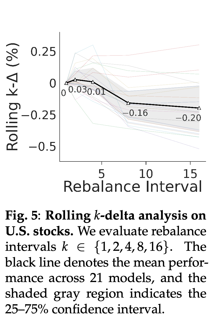
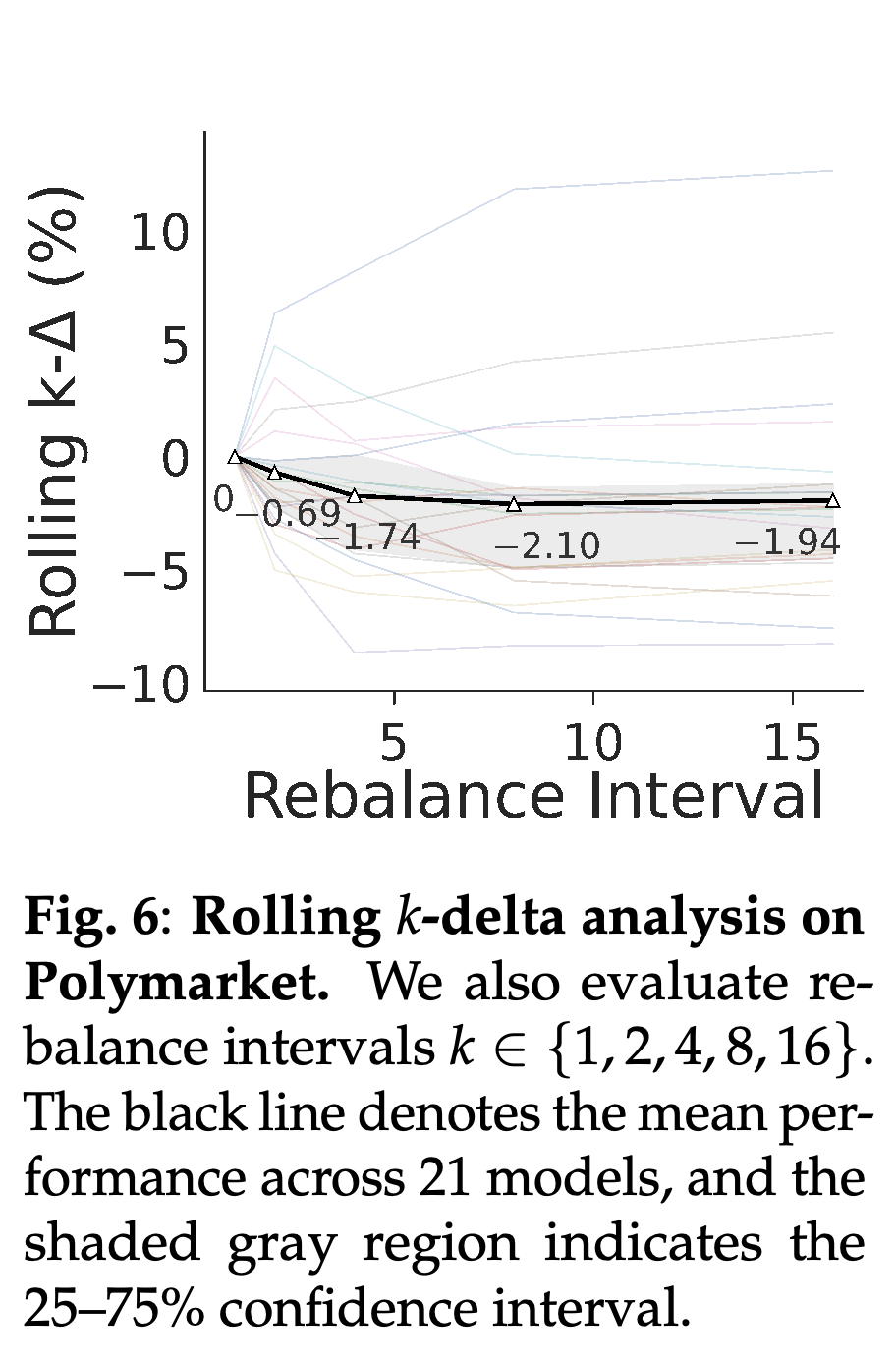
The rolling-k delta analysis measures how cumulative returns change when holdings are replaced by those from k days earlier: \(\Delta_k=CR^{(k)}-CR^{(0)}\), with \(k\in\{1,2,4,8,16\}\). A separate analysis uses another LLM to annotate whether daily explanations mention portfolio positions, price history, or news.

• For stocks, the plotted mean return differences across the tested intervals are 0, 0.03%, 0.01%, −0.16%, and −0.20%. For Polymarket, they are 0, −0.69%, −1.74%, −2.10%, and −1.94%, indicating greater sensitivity to stale holdings in that market.
• The delayed-holdings results support a benefit from timely updating at longer delays. The analysis does not report an explicit random-allocation comparison or significance tests, so it provides narrower evidence than the authors’ claim that the agents do not act randomly.
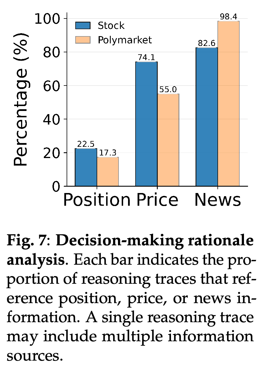
• Stock explanations mention positions in 22.5% of traces, prices in 74.1%, and news in 82.6%; Polymarket explanations mention these in 17.3%, 55.0%, and 98.4%, respectively. A trace can mention multiple sources.
• These annotations measure stated rationales rather than causal dependence on each input. The paper does not report human validation of the annotator.

Mean stock return differences remain close to zero at short delays, including +0.03% at k = 2, before declining to −0.20% at k = 16. The model-specific curves show heterogeneous effects; the shaded 25–75% range is not evidence of a conventional confidence interval for the mean.

Polymarket’s mean differences fall to −0.69%, −1.74%, −2.10%, and −1.94% beyond the initial plotted interval. The larger losses than in stocks indicate greater sensitivity to stale holdings in this evaluation, although the curve does not decrease at every interval.

News appears in 82.6% of stock explanations and 98.4% of Polymarket explanations, while price references are more common in stocks, at 74.1% versus 55.0%. Multiple labels can apply to a single trace, and these frequencies measure explanation content rather than causal input importance.

6. Case Study

The case studies examine selected extreme episodes in stock-market cash allocations and a Russia–Ukraine ceasefire prediction contract. They connect changes in holdings to contemporaneous market conditions and generated explanations, providing qualitative evidence about allocation behavior.

6.1. Cash Asset Dynamics in the U.S. Stock Market

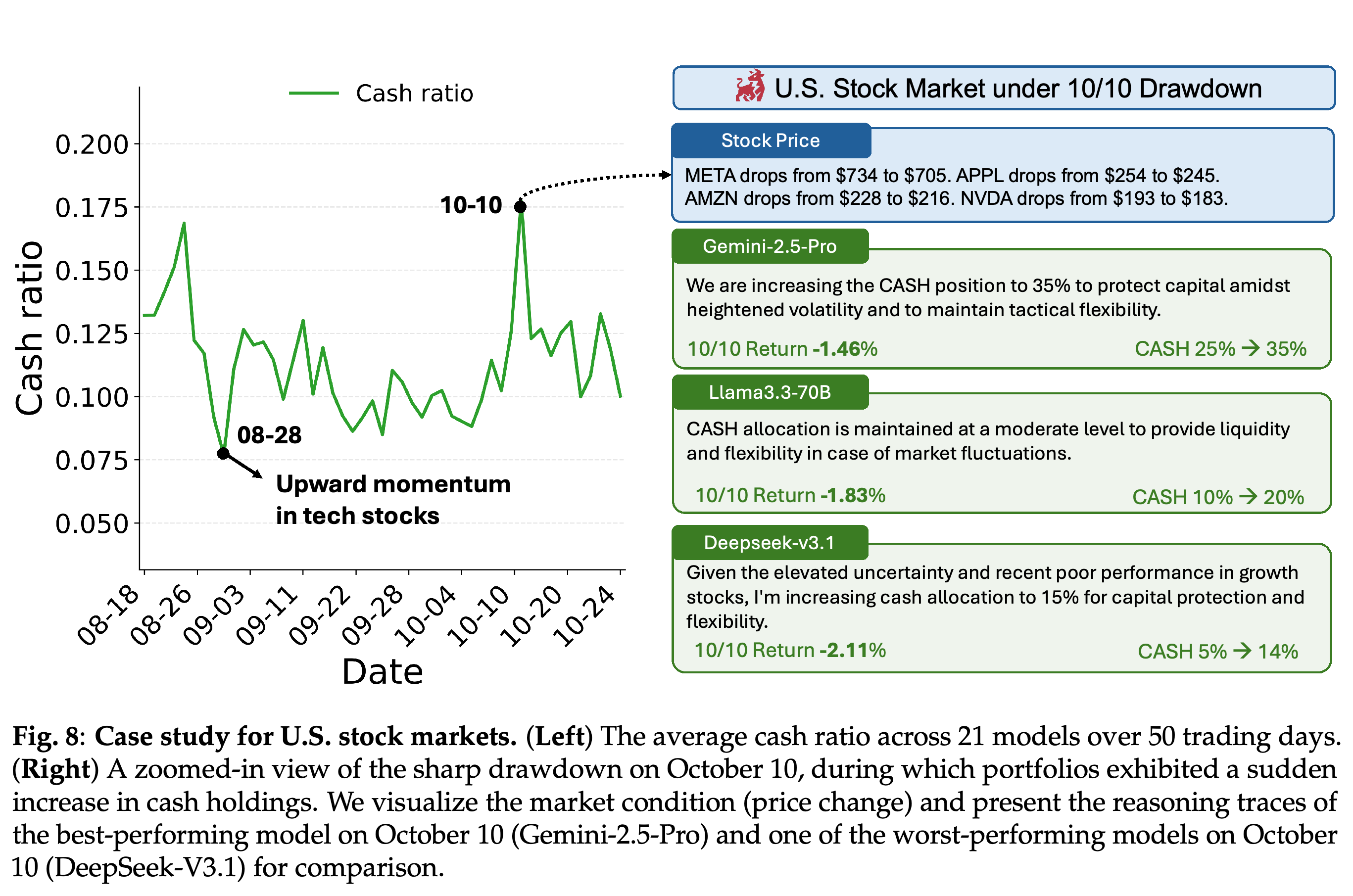
During the technology-stock rally around August 28, mean cash allocation across the 21 models fell from 17% to 7.5% within four trading days. During the October 10 decline, all agents lost money that day and most increased cash holdings, consistent with their stated defensive reasoning.

• The paper reports Tesla falling over 5% and Amazon and NVIDIA falling more than 4% on October 10.
• Figure 8 compares Gemini-2.5-Pro, with a −1.46% daily return and cash increasing from 25% to 35%, Llama3.3-70B, with −1.83% and cash increasing from 10% to 20%, and DeepSeek-V3.1, with −2.11% and cash increasing from 5% to 14%.
• Gemini-2.5-Pro had the smallest loss that day, according to the paper. This selected episode illustrates the relationship between cash exposure and losses without establishing general superiority of its risk management.

Mean cash holdings decline around the August 28 technology rally and rise sharply around October 10. The selected October 10 examples pair higher cash allocations with smaller losses: Gemini-2.5-Pro loses 1.46%, compared with 1.83% for Llama3.3-70B and 2.11% for DeepSeek-V3.1; the comparison does not isolate the effect of cash from other portfolio differences.

6.2. Russia–Ukraine Ceasefire Market in Polymarket Prediction Market

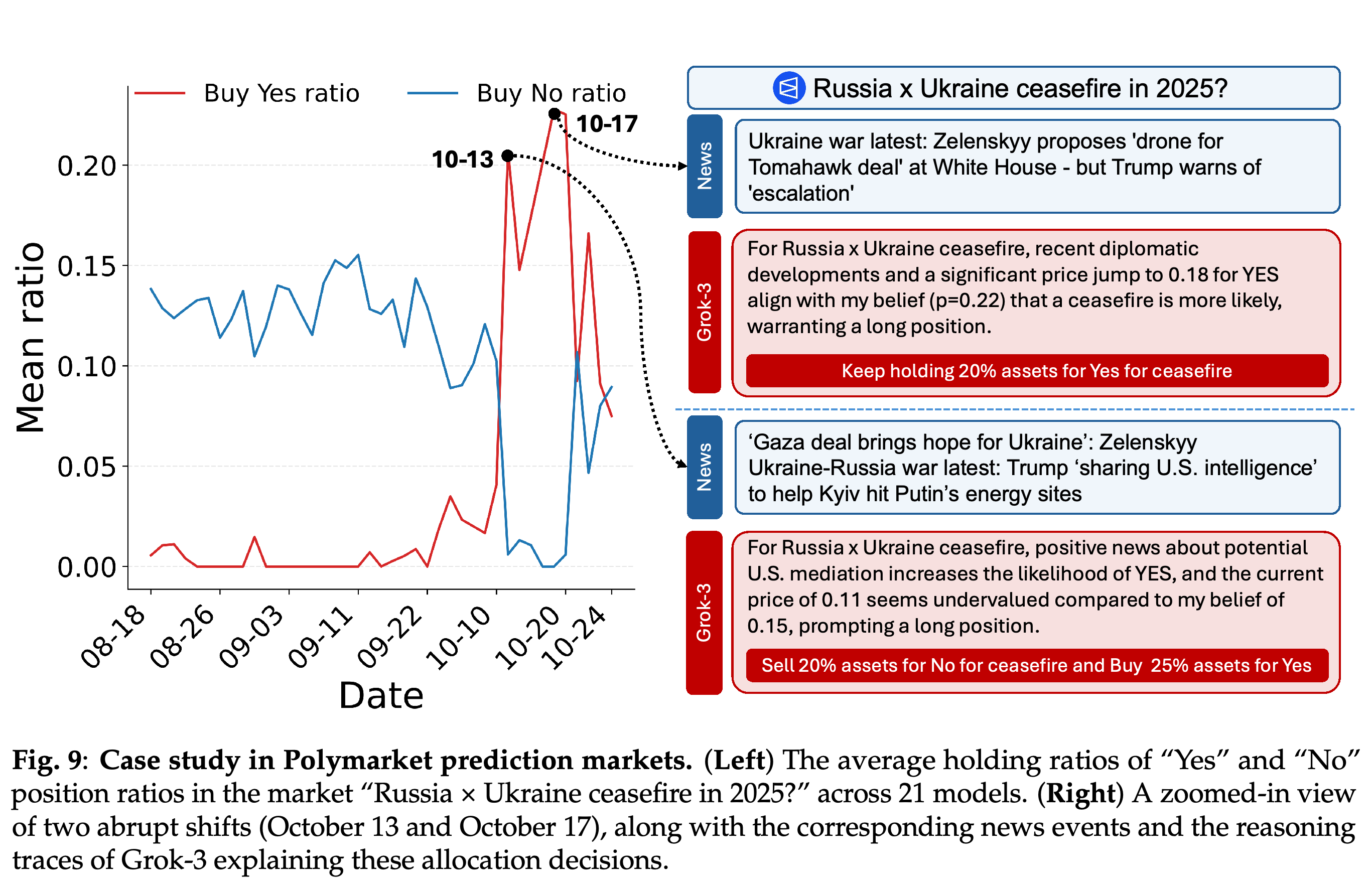
In the market “Russia × Ukraine ceasefire in 2025?”, agents shifted from NO toward YES after optimistic news on October 13, but the paper reports little price movement and no profit from that reaction. On October 17, agents strengthened and held YES positions around news of Zelenskyy’s White House visit, followed by a price increase through October 18 and reported profits.

• Grok-3’s stated event probability rose from 0.15 on October 13 to 0.22 on October 17. Its explanations compared those estimates with YES prices of 0.11 and 0.18, respectively.
• Figure 9 shows mean YES and NO holding ratios across all 21 models together with Grok-3’s explanations for the two dates.
• The authors interpret the first episode as overreaction to weakly decisive news and the second as a better-grounded hold. These interpretations come from selected cases rather than controlled causal tests of the news events.

The mean holding curves show abrupt movement toward YES in the ceasefire market on October 13 and October 17. Grok-3’s accompanying explanations compare its event probabilities of 0.15 and 0.22 with market prices of 0.11 and 0.18, illustrating how stated beliefs connect to allocations in the selected cases.

7. Conclusion

The conclusion presents LiveTradeBench as a setting for studying perception, reasoning, and adaptation under live uncertainty. Its empirical findings include weak transfer of model rankings between markets, weak association between general model scores and trading outcomes, and distinct allocation behaviors associated with prices, news, and portfolio history.

Limitation and Future Work

The authors identify three limitations: omitted trading costs and market frictions, restricted observation and action spaces, and a simplified agent architecture. These constrain the realism of reported returns and the range of financial decisions tested.

• Transaction fees, spreads, and liquidity constraints are omitted, potentially overstating achievable returns for frequently rebalanced portfolios. Proposed extensions include cost models and slippage, differences between assumed and achieved execution prices.
• Agents see limited histories and a small market universe, with news truncated to titles and abstracts. Proposed extensions include longer histories, fuller textual context, and additional markets.
• The basic ReAct setup has limited reasoning depth and temporal abstraction, the ability to organize decisions over longer horizons. Specialized tools, hierarchical memory, collaboration among agents, and reinforcement learning are proposed directions rather than evaluated improvements.

Open-source Application

The released Python package live-trade-bench provides interfaces for data collection, environment setup, and agent construction, while the web application supports live monitoring. The paper supplies https://trade-bench.live, https://github.com/ulab-uiuc/live-trade-bench, and https://pypi.org/project/live-trade-bench/ as access points.

Appendix

• S1. Data Collection and S1.1. Market News Data describe live prices and contextual information associated with ticker symbols or market identifiers; the overview names Google News and Reddit as context sources. Google News queries use \([t-3,t-1]\), with <TICKER> stock news OR <Company Name> for stocks and the market question for Polymarket. Titles, snippets, links, sources, and timestamps are normalized, and entries without valid timestamps are discarded.
• S1.2. Stock Price Data uses yfinance, a finance-data client, with a 10-day lookback ending at t−1, exposing current prices and daily date, adjusted close, and volume. S1.3. Polymarket Price Data uses public market-discovery and price endpoints with the same historical window, removes duplicate event slugs and near-flat series, and normalizes quotes to probabilities in [0, 1]. These windows aim to reduce same-day leakage, although Table S2’s illustrative stock prompt includes a close dated on its decision day, leaving the precise decision-time cutoff unresolved by the example.
• S2. Prompting Details combines dynamic market, news, and account context with a fixed market-specific instruction header. Tables S2 and S3 describe stock context and decision prompts; Tables S4 and S5 describe their Polymarket equivalents, including at most one non-zero YES or NO allocation per question. Outputs contain reasoning and allocations, with weights summing to 1.0 including CASH; the Polymarket prompt asks models to consider costs even though the evaluated environment omits them.
• S3. Model Details uses LiteLLM, a client that routes requests to model providers, with unprefixed names defaulting to Together AI. Standard chat models use temperature = 0.3, a generation-sampling setting, and max_tokens = 16000, an output-length limit; these parameters are omitted for structured reasoning models to retain provider defaults, and outputs are parsed and validated before account updates. S4. Frontend UI Details describes leaderboard, stock, Polymarket, and news views with allocation histories and model inputs and outputs; stock accounts start with 1000 USD and Polymarket accounts with 500 USD.

Brief Thoughts

The main contribution is a shared interface for evaluating sequential decisions across two live information environments; Table 2 makes the dependence of model rankings on the market visible. Evidence for persistent trading skill or causal explanations of behavior is limited by the single 50-day period, omitted execution costs, and absence of input ablations, experiments that remove individual information sources. The results support the conclusion that general model rankings are inadequate proxies for performance in this particular portfolio benchmark. Persistent alpha would require comparisons under matched costs and repeated evaluation across market periods. The leaderboard screenshot includes comparison funds, but Table 2 does not provide a matched statistical analysis against them. The stale-holdings experiment is informative about update timing, while the selected news episodes show that responding to relevant-looking information can still produce unprofitable decisions.