Dynamic Large Concept Models: Latent Reasoning in an Adaptive Semantic Space | Summary

Contents

Summary
1 Introduction
2 Related Work
- 2.1 From Latent Reasoning to Concept-Level Language Modeling
- 2.2 Dynamic Compute Allocation in Language Models
3 Methodology
4 Implementation Details
5 Data
6 Scaling Laws for DLCM
7 Experiments
- 7.1 Main Results
- 7.2 Analysis: Compute Allocation in Concept-Based Models
8 Ablation Studies
9 Conclusion
Contributions
Appendix
Brief Thoughts

This article explains the key points of Dynamic Large Concept Models: Latent Reasoning in an Adaptive Semantic Space.

2025-12-31 (arXiv)
Qu, Xingwei, Wang, Shaowen, Huang, Zihao, Hua, Kai, Yin, Fan, Zhu, Rui-Jie, Zhou, Jundong, Min, Qiyang, Wang, Zihao, Li, Yizhi, et al.
ByteDance Seed, University of Manchester, Mila - Quebec AI Institute, Tsinghua University, M-A-P
Paper

Summary

Dynamic Large Concept Models: Latent Reasoning in an Adaptive Semantic Space proposes a hierarchical next-token prediction architecture that compresses variable-length token segments into latent concepts. A lightweight token encoder and decoder surround a wider concept-level Transformer, shifting expensive computation to a shorter sequence.
DLCM combines representation-based boundary detection, globally regularized compression, a compression-aware scaling law, and decoupled µP for unequal-width modules. The practical configuration uses R = 4; the main comparison trains a 2.3B-parameter DLCM and a 1.3B-parameter baseline on 1T tokens, with inference FLOPs described as comparable rather than parameters matched.
The paper reports 43.92% versus 41.23% average accuracy and a +2.69% improvement across 12 zero-shot benchmarks, but the displayed Table 2 rows yield approximately 42.24% versus 41.23% under an unweighted arithmetic mean. DLCM improves eight task scores and regresses on BoolQ, RACE, MMLU, and CMMLU; the results support task-dependent gains, while the aggregate discrepancy limits confidence in the headline magnitude.

1 Introduction

The motivating problem is non-uniform information density: standard language models apply the same depth to predictable spans and difficult semantic transitions. DLCM introduces an intermediate granularity between tokens and predefined sentences, defining a concept operationally as a variable-length latent segment rather than a guaranteed linguistic or human-interpretable unit.

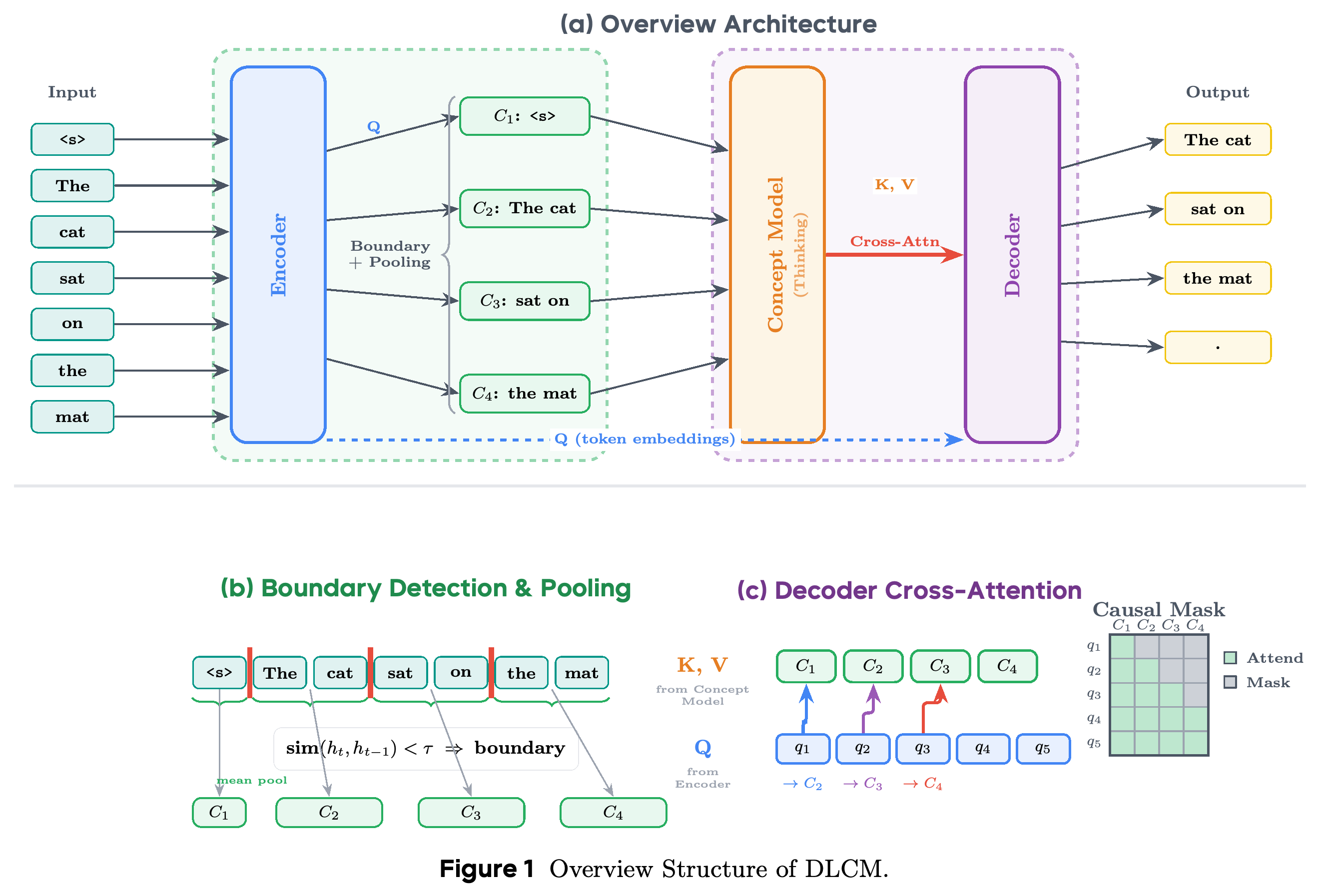
The four-stage pipeline comprises encoding, dynamic segmentation and pooling, concept-level reasoning, and token-level decoding, as illustrated in Figure 1.
The introduction claims up to 34% FLOPs reduction and improved benchmark accuracy through compute redistribution. Architectural savings should be distinguished from the main comparison, which increases total parameters while describing inference FLOPs as matched.

DLCM architecture with boundary detection, mean pooling, concept-level processing, and decoder cross-attention.

Related work places DLCM at the intersection of continuous latent reasoning, concept-level language modeling, and adaptive computation. Its proposed distinction is to combine representation-based segmentation with token-level autoregressive prediction rather than use fixed sentence embeddings or focus on byte-level modeling.

2.1 From Latent Reasoning to Concept-Level Language Modeling

COCONUT feeds hidden states between reasoning steps without generating intermediate tokens, whereas Large Concept Models operate over sentence embeddings produced and decoded by frozen modules. DLCM replaces the fixed sentence prior and separately pretrained encoder–decoder requirement with trainable token modules and variable-length latent segments.

The discussion attributes reduced interpretability and difficulties with precise symbolic manipulation to continuous latent reasoning. These are observations about prior work, not direct DLCM evaluations.
The claims concerning SONAR, generation in 200+ languages, and approximately 10× sequence reduction describe prior Large Concept Models, not demonstrated DLCM capabilities.

2.2 Dynamic Compute Allocation in Language Models

Universal Transformers adapt depth through recurrence and halting, while Mixture of Experts routes tokens to subsets of parameters. H-NET is the closest architectural precedent because it learns boundaries and hierarchically processes compressed chunks; DLCM adapts this principle to token-level next-token prediction.

3 Methodology

The methodology separates token representation, segment formation, computation over concepts, and reconstruction of token predictions. Section 3.3 qualifies the broader end-to-end learning claim: the discrete segmentation decision is intentionally decoupled from the language-modeling loss to avoid competing optimization objectives.

3.1 Overview

The formal pipeline is (H=E(x),\quad C=\Phi(H),\quad Z=M(C),\quad \hat y=D(\Psi(H,Z))). E encodes tokens, Φ segments and pools them, M processes the concept sequence, and Ψ supplies concept-conditioned token features to decoder D.

3.2 Encoding

A standard causal Transformer encoder maps the input sequence into contextual token representations with width dtoken. These representations support both boundary detection and token-level decoding, retaining a direct path for local information around the compressed backbone.

3.3 Dynamic Segmentation

Dynamic segmentation uses adjacent projected representations to estimate boundary probabilities, then mean-pools each contiguous segment and projects it into the wider concept space. The Global Parser regularizes boundary rates across the distributed batch rather than forcing each sequence to meet the same compression ratio.

3.3.1 Boundary Detection: qt = Wqht and kt = Wkht; pt = (1 − cos(qt−1, kt))/2, with p1 = 1. Training samples Bernoulli boundaries after temperature sharpening by α; inference uses bt = [pt ≥ 0.5].
3.3.2 Concept Formation via Pooling: craw_k = (1/|Sk|) Σt∈Sk ht and ck = Wup craw_k. Each segment contributes one concept regardless of its token length.
3.3.3 Adaptive Compression via Global Load Balancing: expected and realized boundary rates Gglobal and Fglobal are synchronized through AllReduce. Equation 10 defines Laux = R/(R − 1) [(R − 1) Fglobal Gglobal + (1 − Fglobal)(1 − Gglobal)] − 1, intended to maintain a global boundary rate of 1/R while permitting local variation.

3.4 Concept-Level Reasoning

The computational core is a standard causal Transformer with Lconcept layers operating on the shorter concept sequence. Compression reduces the sequence length seen by this module, permitting a wider, higher-capacity backbone; interpreting its computation as high-level reasoning is the paper’s architectural hypothesis rather than a separately supervised capability.

3.5 Token-Level Decoding

Token-level decoding applies a lightweight concept-smoothing module and then cross-attends from encoder token features to processed concepts. Separate projections reconcile dtoken and dconcept, and the attention output is projected back to token width with an encoder residual connection.

3.5.1 Concept Smoothing: Z̃ = S(Z) integrates adjacent concepts to reduce artifacts introduced by hard pooling. The section does not specify the smoothing module’s architecture.
3.5.2 Causal Cross-Attention: the stated mask restricts token t to concepts up to j(t) = Σi=1…t bi. Equation 14 gives Ψ(H, Z) = Softmax(QK⊤/√dhead + M)VWO + H.
The equations do not explicitly explain how a token’s access to its pooled current segment excludes later tokens from that segment. Causal masking is stated, but the segment-completion or alignment convention needs clarification.

3.6 Training Objective

Training minimizes L = LCE + λLaux, combining output-token cross-entropy with compression load balancing. Both objectives appear in the total loss, while the discrete segmentation decision remains decoupled from the language-modeling loss as described in Section 3.3.

4 Implementation Details

Implementation uses packed Variable Length training from FlashAttention so global compression statistics span diverse tokens. RMSNorm is applied to attention queries and keys to stabilize interactions between token-level and concept-level representations with different statistical properties.

4.1 Efficient Cross-Attention via Concept Replication

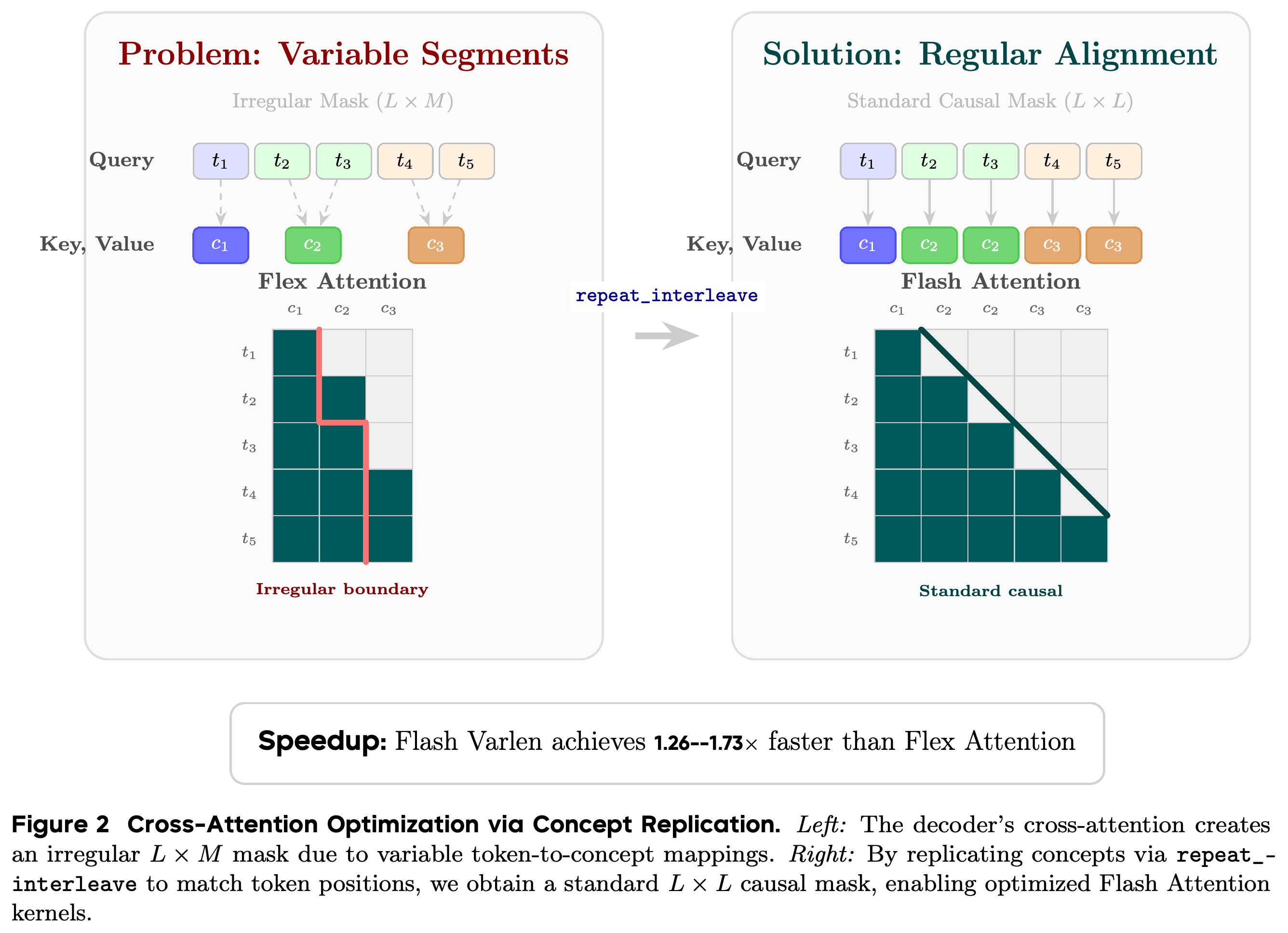
Concept replication replaces an irregular token-to-concept attention layout with a token-aligned key/value sequence. The implementation uses repeat_interleave(K, segment_lengths) and repeat_interleave(V, segment_lengths), enabling Flash Attention Varlen with a standard causal mask instead of Flex Attention’s irregular mask.

Figure 2 illustrates the conversion from an L × M layout to an L × L layout whose key/value vectors are constant within each segment.
Replication increases key/value storage to obtain a more regular kernel layout. Because repeated keys affect softmax multiplicity, the implementation should not be assumed to preserve the unreplicated concept-level attention weights without further explanation.

Conversion of irregular token-to-concept attention into token-aligned causal attention through repeat_interleave.

4.2 Performance Benchmarks

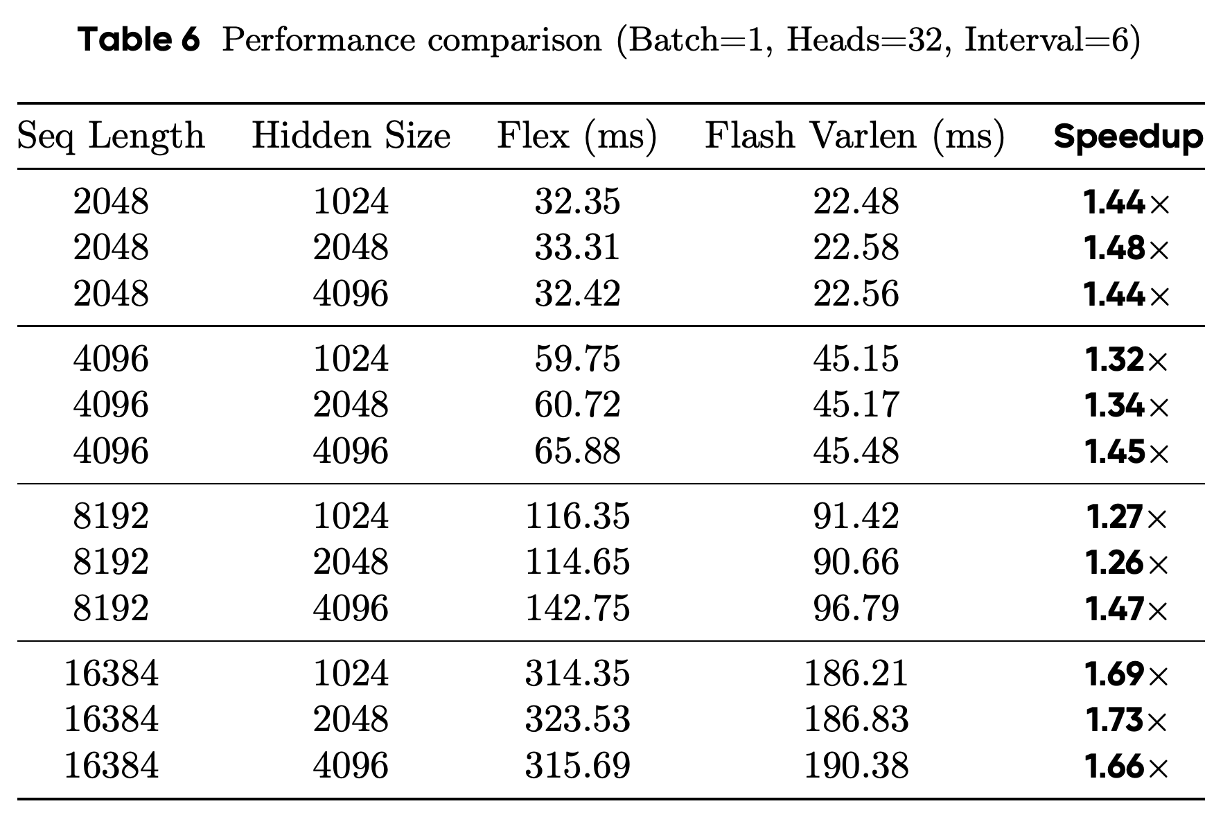
The independent kernel benchmark tests sequence lengths 2048, 4096, 8192, and 16384 with hidden sizes 1024, 2048, and 4096. Table 6 specifies Batch=1, Heads=32, Interval=6; these are profiling configurations, not necessarily the actual DLCM module dimensions.

All 12 measured configurations favor Flash Attention Varlen, with speedups from 1.26× to 1.73×.
These measurements concern kernel execution, not end-to-end autoregressive generation latency, serving throughput, or memory consumption.

Flex Attention and Flash Attention Varlen kernel timings for 12 sequence-length and hidden-size configurations.

4.3 Key Observations and Analysis

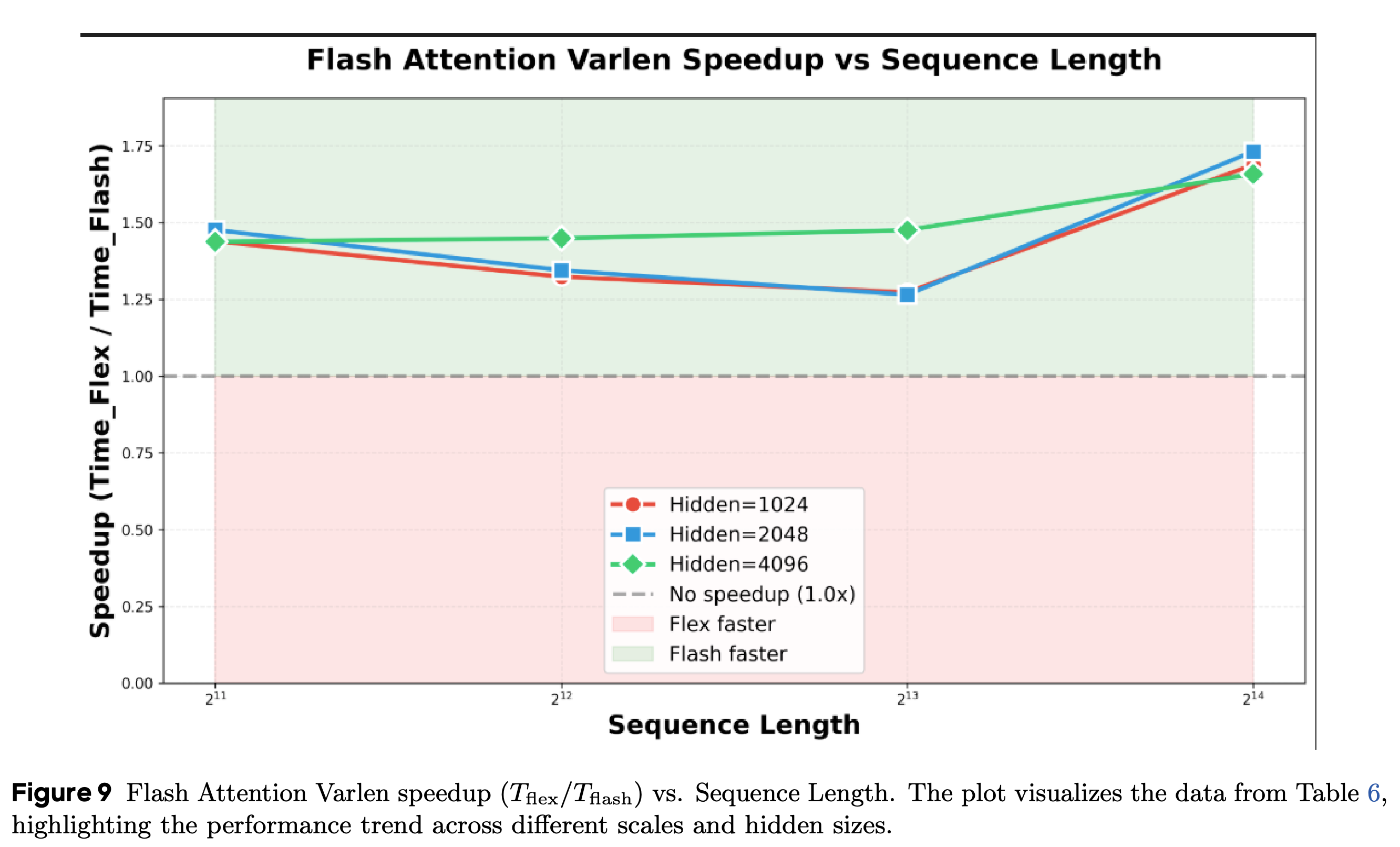
Flash Attention Varlen reaches its largest measured advantage at 16384 tokens: 1.69×, 1.73×, and 1.66× for hidden sizes 1024, 2048, and 4096. Figure 9 and Table 6 show non-monotonic scaling at intermediate lengths, supporting a strong long-sequence advantage rather than continuously increasing speedup.

At hidden size 2048, speedup decreases from 1.48× at 2048 tokens to 1.34× at 4096 and 1.26× at 8192 before reaching 1.73× at 16384.
The authors attribute the advantage to regular memory access and reduced dynamic-mask overhead, but the timings do not separately measure those effects.
The claim of nearly identical behavior across widths is approximate: at 8192 tokens, hidden size 4096 achieves 1.47× versus 1.27× and 1.26× for the smaller widths.

Flash Attention Varlen speedup relative to Flex Attention across sequence lengths and hidden sizes.

5 Data

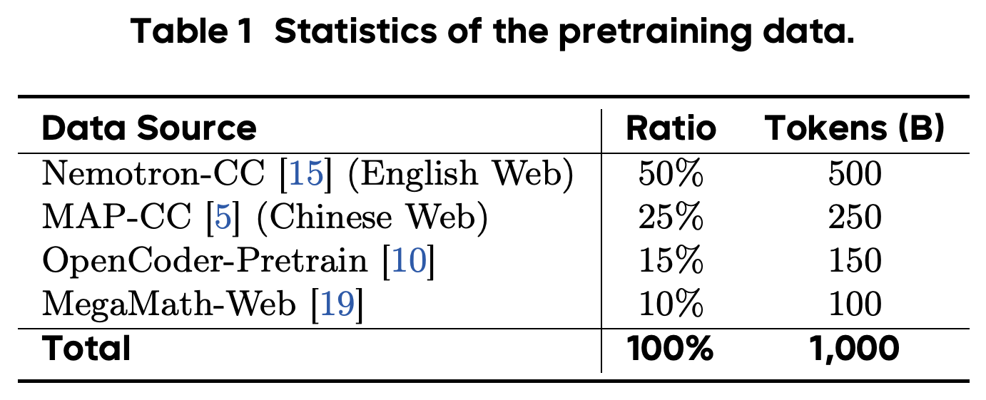
The corpus contains 1,000B tokens from open-source English and Chinese web text, code, and mathematics, tokenized with the DeepSeek-v3 tokenizer. Table 1 allocates 50%/500B to Nemotron-CC, 25%/250B to MAP-CC, 15%/150B to OpenCoder-Pretrain, and 10%/100B to MegaMath-Web.

The authors use domain diversity to provide broad language coverage and expose segmentation to different information densities, without aggressive filtering.
The data section describes an entirely open-source corpus, whereas Section 7.1 calls the dataset proprietary. The paper does not reconcile these descriptions.

Pretraining sources, mixture ratios, and token counts.

6 Scaling Laws for DLCM

The scaling study addresses heterogeneous-module optimization and architectural allocation under compression. It introduces component-specific µP scaling before fitting a loss model that separates token parameters, concept parameters, training data, and compression ratio.

6.1 Decoupled µP for Heterogeneous Architectures

Decoupled µP defines independent width multipliers stoken = dtoken/dbase and sconcept = dconcept/dbase. Hidden-weight initialization variances, hidden-layer learning rates, and AdamW ϵ scale inversely with the corresponding module width; embeddings retain fixed initialization variance and learning rate, and output logits are divided by stoken.

6.1.1 Formulation of µP: ηE,D = ηbase_token/stoken and ηM = ηbase_concept/sconcept allow token and concept modules to widen independently. Biases and embeddings use the fixed learning rate ηbase_others.
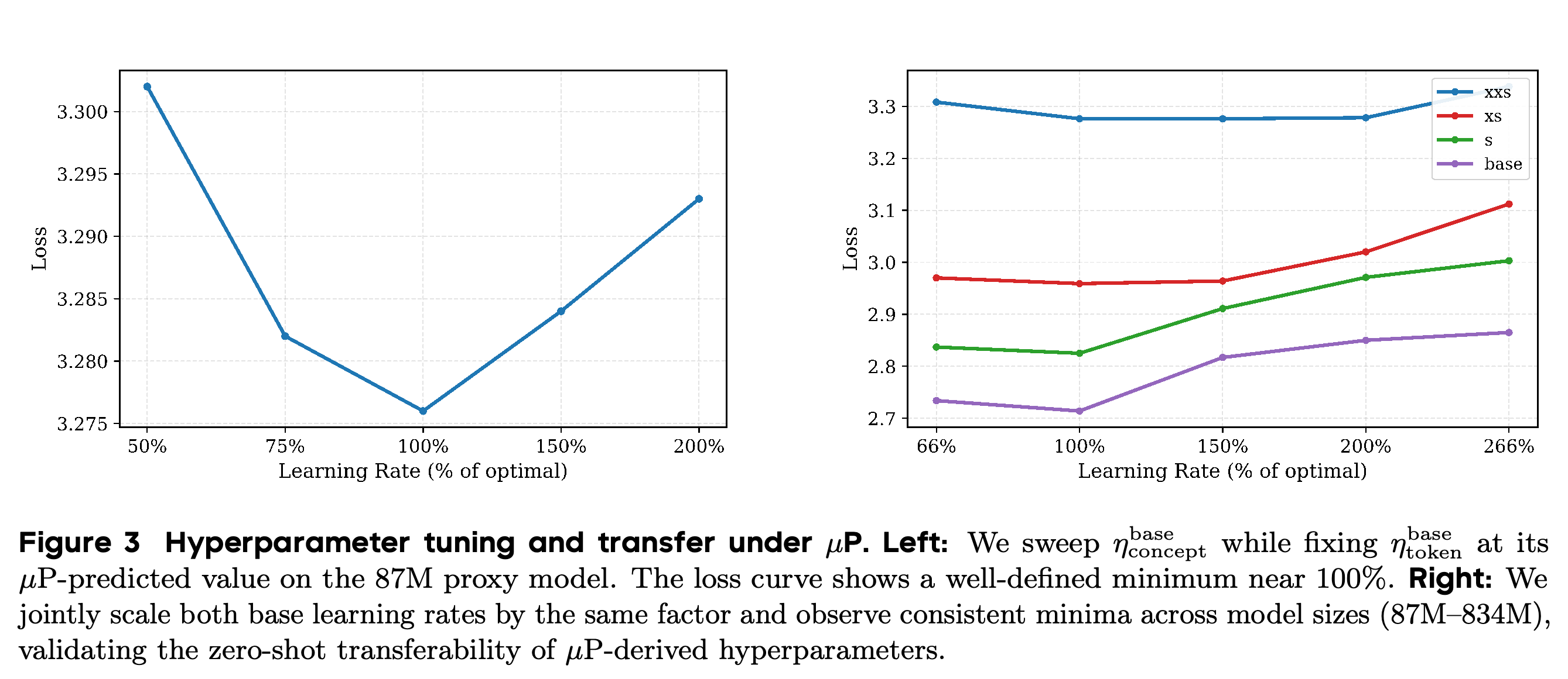
6.1.2 Hyperparameter Tuning and Verification: coordinate descent on an 87M proxy uses multiplicative factors {0.5, 0.75, 1.5, 2.0}. The selected token and concept base learning rates are approximately equal, although their actual rates differ after width scaling.
Following Yang et al., transfer is checked at 274M, 468M, and 834M parameters by jointly perturbing the transferred base rates. Figure 3 shows minima near the predicted settings, supporting transfer across the tested model widths rather than establishing it across every compression regime.

Proxy-model learning-rate tuning and transfer checks under decoupled µP.

6.2 Scaling Law Formulation

The scaling grid varies P ∈ {30%, 50%, 70%} and R ∈ {2, 4, 8}, with a stated 200B-token training budget and model scales 274M, 468M, and 833M. Equation 22 extends the Chinchilla framework by separating token-capacity, compression-dependent concept-capacity, and data terms, with globally shared δ1, δ2, and γ.

6.2.2 Mathematical Formulation: L(N, D, R, P) = E0 + Atoken/[N(1 − P) + ttoken]^δ1 + Aconcept R^γ/[NP + tconcept]^δ2 + Adata/[D + tdata]^α. P is the concept-layer parameter fraction and E0 the irreducible loss floor; only scale-independent offset terms are allowed to vary across configurations.
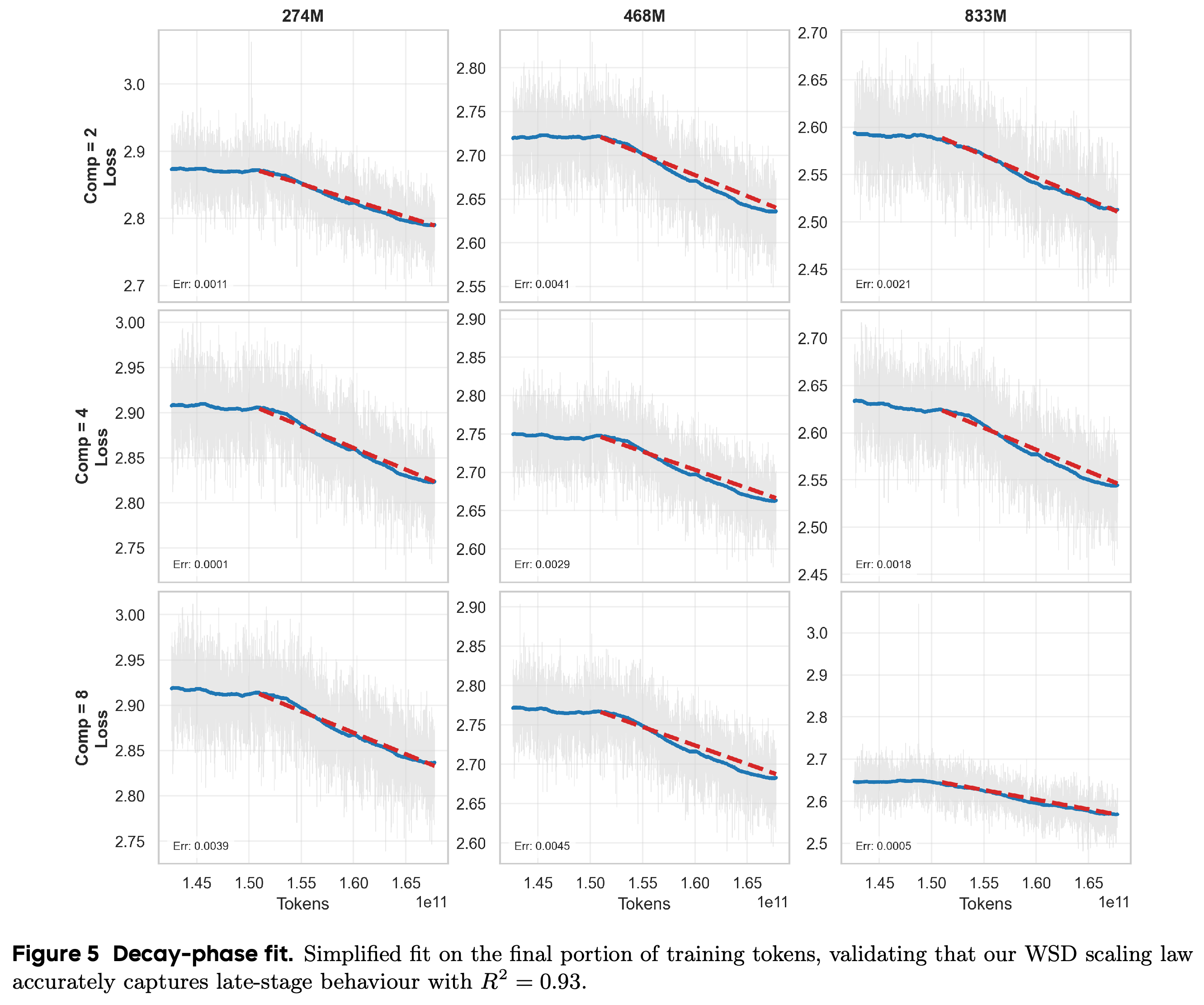
6.2.3 Decay-Phase Power Law: the paper calls its WSD protocol Weight-Sharing-and-Decay and fits Δdecay = k Lstable^a R^b N^c over the 90%–99% token window. Log-linear regression gives R² = 0.93.
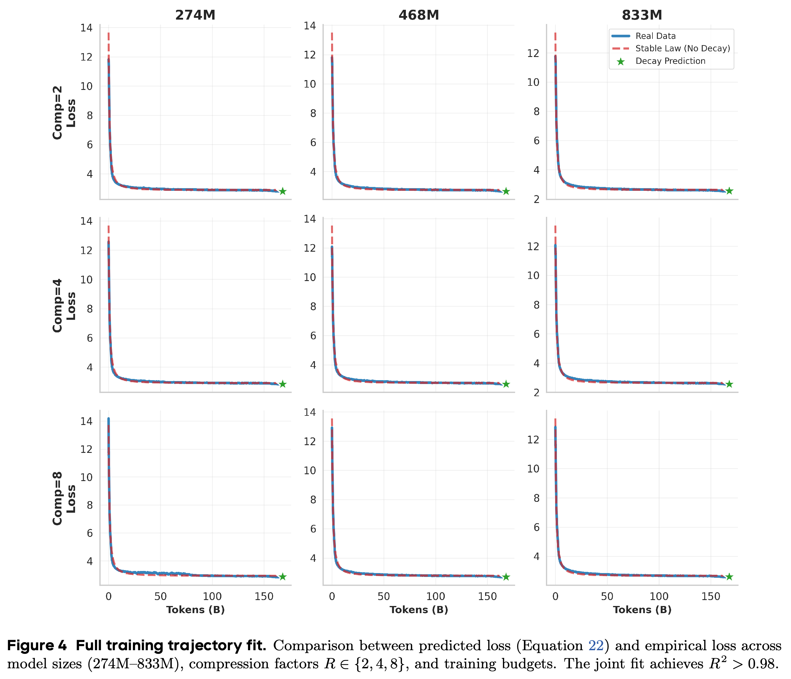
Figures 4 and 5 compare predicted and empirical trajectories, reporting R² > 0.98 for the full-trajectory fit and R² = 0.93 for late-stage decay.

Full-training loss trajectories and compression-aware scaling-law predictions.

Late-stage empirical loss and decay-phase predictions across model sizes and compression ratios.

6.3 Optimal Configuration Analysis

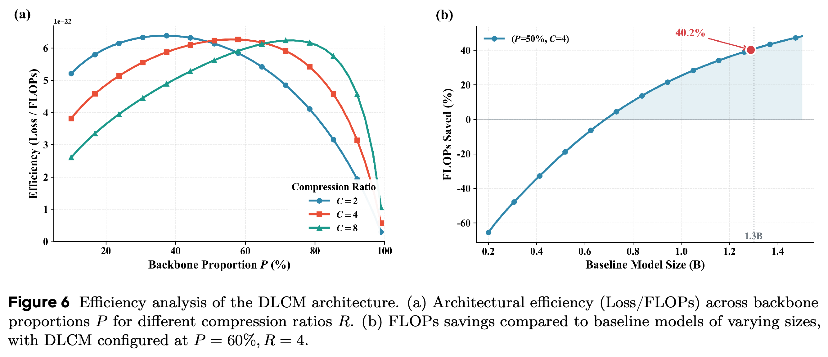
Figure 6(a) shows the plotted efficiency peak moving toward larger concept-backbone fractions P as compression R increases. The authors select R = 4 as a practical compromise between segmentation granularity, training stability, and computational efficiency, citing Appendix A’s qualitative examples.

The appendix illustrates segmentation behavior but does not quantitatively establish that R = 4 is optimal.
Figure 6(b) has inconsistent configuration labels: its caption states P = 60%, R = 4, whereas the legend states P = 50%, C = 4. Its marked 40.2% saving at a 1.3B baseline also differs from the introduction’s up-to-34% figure; their relationship is not explained.

Architectural allocation efficiency and estimated FLOPs savings relative to baseline model size.

6.4 Scaling Law Validation and Verification

The estimator combines full-training trajectories with late-stage decay and emphasizes observations near convergence. Section 6.4 reports fitting on 100B-token trajectories, validation against 1T-token limits, fitting error below 0.05, and an effective compute multiplier of approximately 1.4 compared with a stated baseline factor of 1.34.

These conditions differ from the 200B-token grid in Section 6.2.1. The relationship between the fitting, training, and extrapolation budgets is not fully explained.
Figures 4 and 5 show trajectories below 1T tokens, so their visual agreement does not by itself verify the claimed 1T extrapolation accuracy.

7 Experiments

Experiments comprise a 1T-token downstream comparison and a separate 100B-token position-wise loss analysis. The first assesses task accuracy with a larger compressed backbone; the second examines prediction loss at different positions within segments.

7.1 Main Results

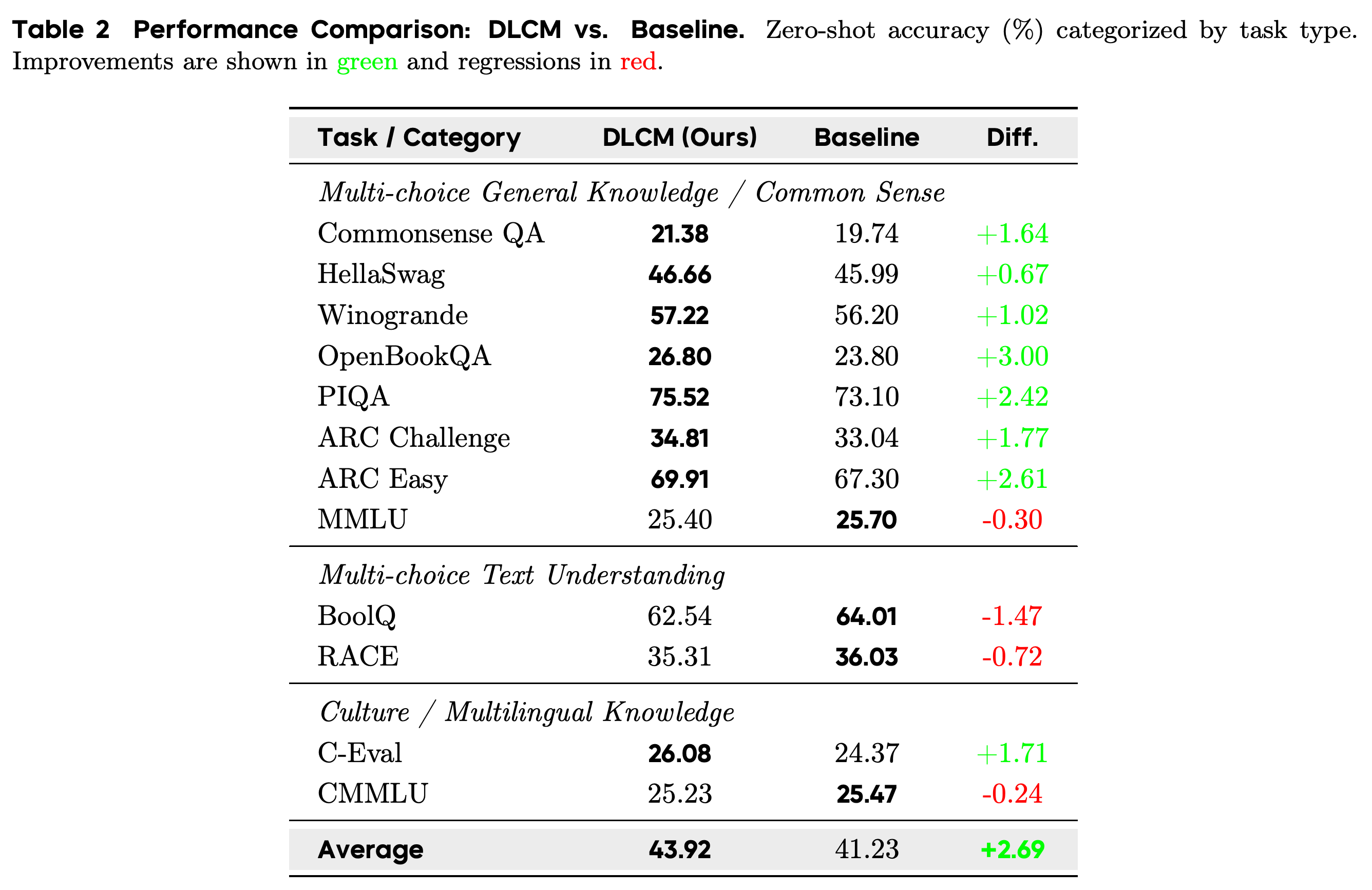
Table 2 reports improvements on Commonsense QA (+1.64), HellaSwag (+0.67), Winogrande (+1.02), OpenBookQA (+3.00), PIQA (+2.42), ARC Challenge (+1.77), ARC Easy (+2.61), and C-Eval (+1.71), all in accuracy percentage points. Regressions occur on MMLU (−0.30), BoolQ (−1.47), RACE (−0.72), and CMMLU (−0.24), showing a task-dependent rather than uniform advantage.

The reported aggregate is 43.92% versus 41.23%, or +2.69%. An unweighted arithmetic mean of the 12 displayed rows gives approximately 42.24% versus 41.23%, a difference of approximately 1.01 percentage points; the paper supplies no alternative aggregation rule.
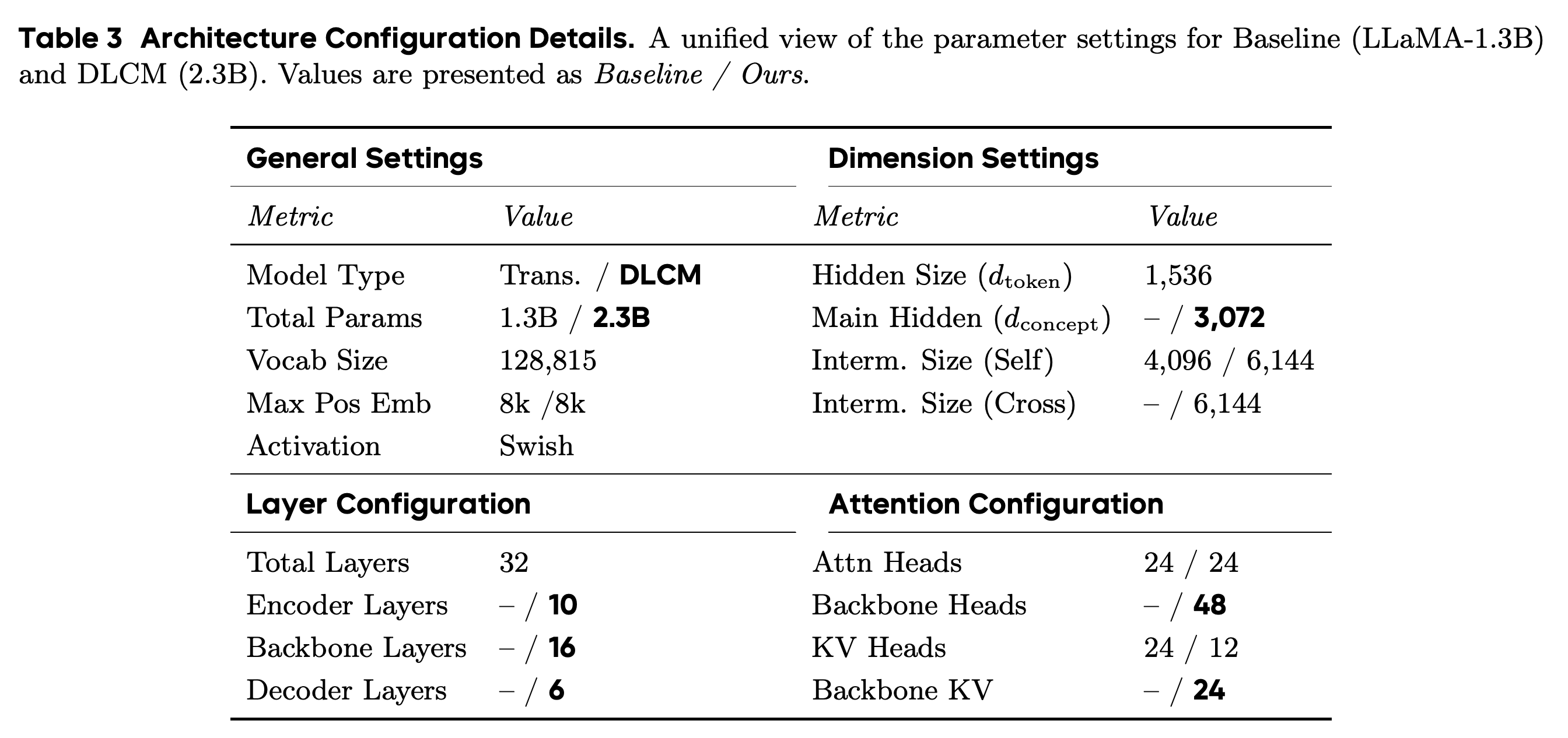
Section 7.1 initially calls the baseline parameter-matched, but its later discussion and Table 3 specify 2.3B versus 1.3B parameters. The intended comparison is described as comparable inference FLOPs, with extra parameters concentrated in the compressed concept backbone.
Table 3 specifies dtoken = 1,536, dconcept = 3,072, vocabulary size 128,815, 8k maximum positions, and 32 total layers. DLCM allocates 10 encoder, 16 backbone, and 6 decoder layers, with 24 token attention heads and 48 backbone heads.
Both models are trained from scratch on 1T tokens. The paper says global batch size, learning rate, and sequence length follow the LLaMA paper but does not give their numerical values in this section or report uncertainty for the task differences. Its explanations involving reasoning, lexical fidelity, and factual recall remain hypotheses rather than isolated experimental findings.

Zero-shot benchmark accuracies for DLCM and the baseline, grouped by task type.

Baseline and DLCM parameter counts, dimensions, layer allocations, and attention configurations.

7.2 Analysis: Compute Allocation in Concept-Based Models

The loss analysis compares a concept model and baseline described as sharing a 1.3B-parameter backbone architecture and an identical 100B-token training subset. It aligns losses from 600 randomly selected validation samples by relative position within a concept and plots the first 20 positions in Figure 7.

The authors describe a U-shaped improvement pattern, with lower loss near early and late positions and mixed or worse performance inside concepts.
The bars qualify the claimed boundary ranges: positions 2 and 18 show degradation, position 14 shows improvement, and some interior differences are near zero. The evidence establishes non-uniform positional effects, not an uninterrupted boundary advantage.
Position measured from a concept’s start does not identify distance to its ending boundary. Without position-specific counts or uncertainty, the plot supports a prediction-loss trade-off more directly than it establishes causal compute allocation or improved global coherence.

8 Ablation Studies

The ablations examine boundary-learning stability, the scope of compression regularization, and domain-dependent segmentation. They provide evidence for controllable compression and variable segment lengths, but do not independently establish that the boundaries correspond to optimal semantic units.

8.1 Analysis: End-to-End Discrete Boundary Learning vs. Decoupled Segmentation

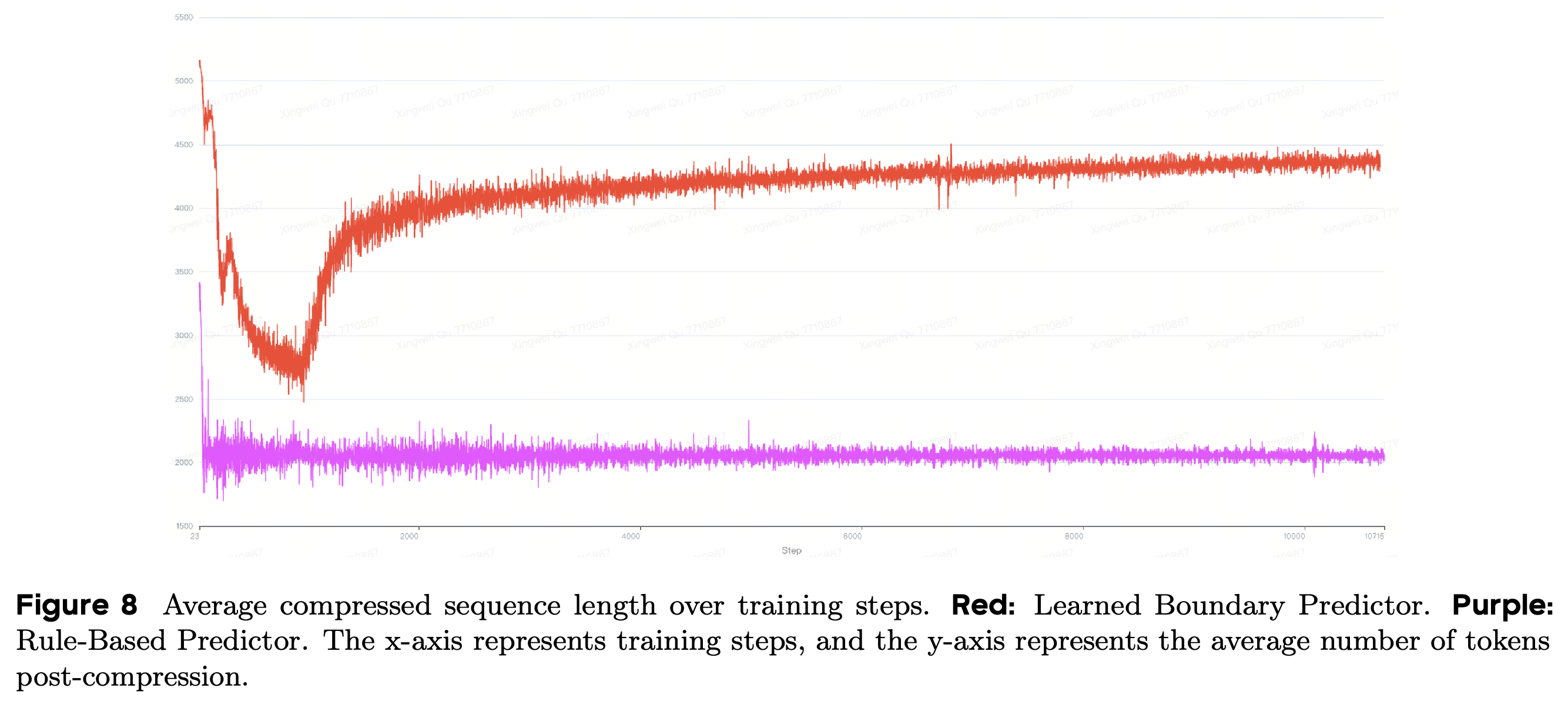
For input length L = 8192, Figure 8 contrasts a learned boundary predictor with a cosine-similarity rule operating on learned representations. The learned predictor initially compresses to approximately 2000 positions but drifts toward approximately 4300, or 1.9× compression; the decoupled rule remains near 2000, or 4× compression.

The authors attribute drift to cross-entropy gradients favoring information retention and overpowering the auxiliary compression gradient. Equation 24 expresses this explanation, but Figure 8 measures compressed length rather than gradient magnitudes.
The rule-based ablation inserts boundaries when pt = (1 − cos(ht, ht+1))/2 exceeds τ. This differs in indexing, projection detail, and threshold description from Section 3.3.1; the paper does not fully specify the relationship between the formulations.

Training evolution of compressed sequence length for learned and decoupled rule-based boundary prediction.

8.2 Global Regularization via Gradient Accumulation

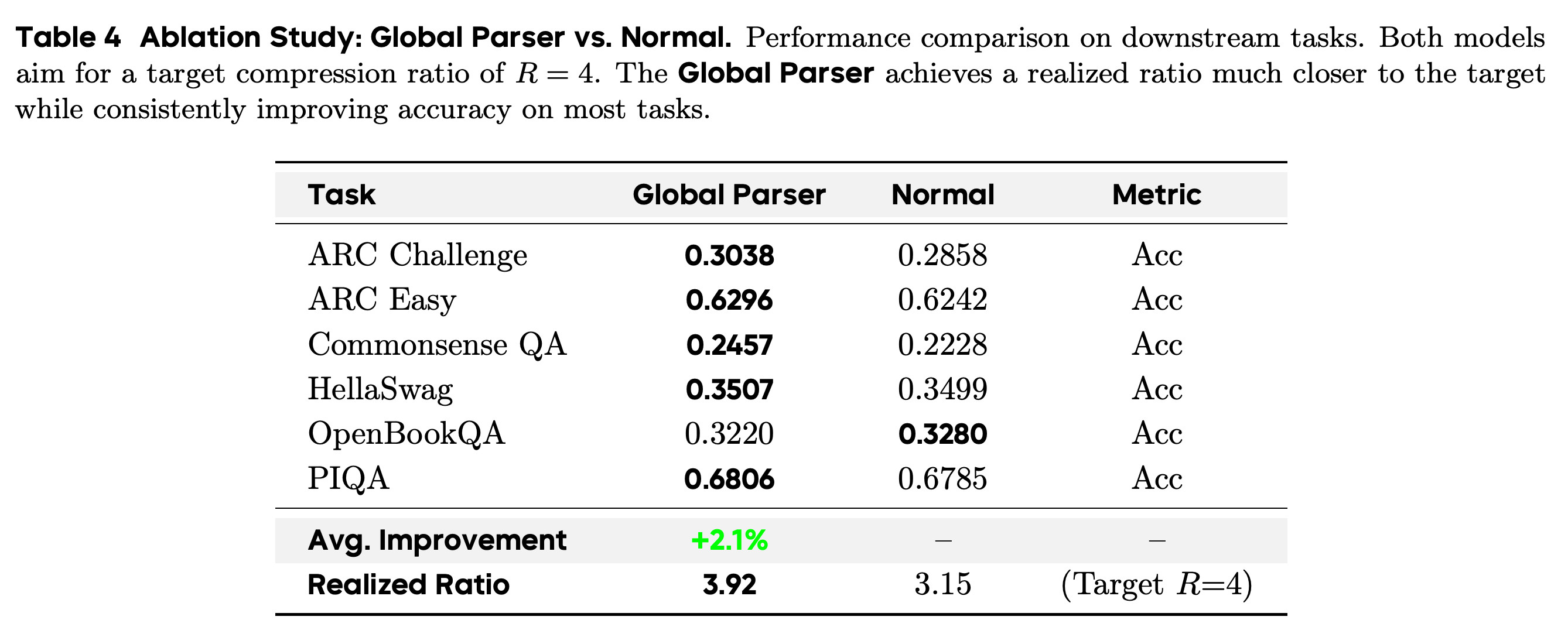
Global regularization aggregates boundary statistics across K micro-batches rather than constraining each sequence separately. Table 4 compares two 2.3B-parameter models trained for 1T tokens and reports realized compression ratios of 3.92 for Global Parser and 3.15 for Normal, against the table’s stated target R = 4.

Global Parser improves five of six listed tasks: ARC Challenge 0.3038 versus 0.2858, ARC Easy 0.6296 versus 0.6242, Commonsense QA 0.2457 versus 0.2228, HellaSwag 0.3507 versus 0.3499, and PIQA 0.6806 versus 0.6785. OpenBookQA declines from 0.3280 to 0.3220.
The setup sentence specifies R = 2, while the subsequent discussion and Table 4 specify R = 4. The experimental compression target is therefore inconsistent in the source.
Table 4 reports an average improvement of +2.1% without defining its aggregation. The displayed scores yield approximately +0.72 percentage points under an unweighted absolute-accuracy average, so +2.1% should not be presented as a verified percentage-point gain.

Global Parser and per-sequence regularization results, including realized compression ratios.

8.3 Content-Adaptive Compression Benefits

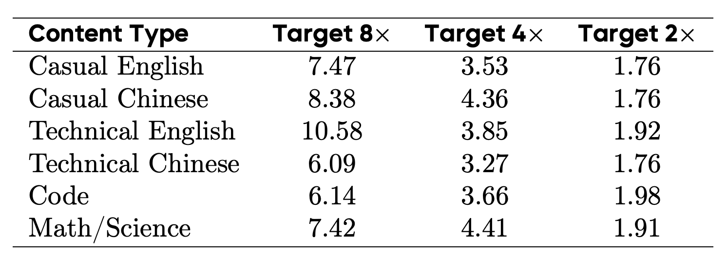
Table 5 shows that achieved tokens per concept vary by content type under a shared target. At target 8×, Technical English reaches 10.58 tokens per concept, Technical Chinese 6.09, and Code 6.14; at target 4×, the six domain averages range from 3.27 to 4.41.

For targets 8×/4×/2×, Casual English gives 7.47/3.53/1.76; Casual Chinese 8.38/4.36/1.76; Technical English 10.58/3.85/1.92; Technical Chinese 6.09/3.27/1.76; Code 6.14/3.66/1.98; and Math/Science 7.42/4.41/1.91.
The domain differences demonstrate flexible granularity rather than rigid per-sequence compression. The table does not directly measure information density, information retention, or segmentation optimality.

Average tokens per concept across six content types at target compression ratios 8×, 4×, and 2×.

9 Conclusion

The conclusion identifies adaptive granularity, compression-aware architectural allocation, and heterogeneous-module optimization as DLCM’s main contributions. The experiments support stable compression in the reported ablation, hyperparameter transfer within the tested widths, and mixed downstream accuracy gains; they do not establish universal reasoning improvements or end-to-end serving efficiency.

Contributions

The Contributions section distinguishes leading authors, individual responsibilities, core contributors, other contributors, and corresponding authors. These statements document project credit rather than provide additional experimental evidence.

Leading Authors

The leading authors are Xingwei Qu, Shaowen Wang, Zihao Huang, and Ge Zhang.

Leading Author Contributions

Xingwei Qu is credited with fundamental ablations and most engineering implementation; Shaowen Wang with MuP implementation and hyperparameter tuning; Zihao Huang with noise-based boundary prediction techniques; and Ge Zhang with the original idea, demo prototype, and key Global Parser technique.

Core Contributors

Kai Hua is credited with open-source training-data construction, Fan Yin with SGLang implementation and optimization, and Rui-Jie Zhu with bug resolution and a proposal to replace the encoder with DLCM. Jundong Zhou and Qiyang Min contributed to project development and implementation.

Other Contributors

Other contributors are Zihao Wang, Yizhi Li, Tianyu Zhang, He Xing, Zheng Zhang, Yuxuan Song, Tianyu Zheng, and Zhiyuan Zeng.

Corresponding Authors

The Contributions section lists Chenghua Lin, Ge Zhang, and Wenhao Huang as corresponding authors. The title page separately gives correspondence contacts xingwei.qu@bytedance.com and zhangge.eli@bytedance.com.

Appendix

A Appendix: Segmentation Examples at Different Compression Ratios presents A.1 Casual English Text, A.2 Python Code, and A.3 Mathematical Text. The source labels identify 90, 87, and 95 original tokens respectively, with segment counts of 11/35/56, 12/29/58, and 13/32/61 under Compression 8×/4×/2×.
The examples show progressively finer splitting of coffee-related prose, SimpleTextDataset code, and an exposition of Euler’s formula, e^ix = cos(x) + i sin(x). Boundaries sometimes split contractions, identifiers, or formulas, and several displays omit parts of the original passage. The stated segment counts do not consistently match the visible separator-delimited spans, so they should be retained as source labels rather than verified counts.

Brief Thoughts

DLCM provides a concrete architecture for assigning expensive computation to a compressed latent sequence while retaining token-level input and output interfaces. The compression-stability ablation, domain-varying segment lengths, and µP transfer experiments support this design more directly than they support a semantic or reasoning interpretation of its concepts. The headline benchmark gain requires reconciled aggregation, and the main result should be described as a larger-parameter, comparable-inference-FLOPs comparison rather than parameter-matched. Reproducibility requires consistent compression targets and scaling budgets, explicit causal segment alignment, clarification of replication’s attention weights, and end-to-end latency and memory measurements. BoolQ and RACE regressions are consistent with the proposed granularity trade-off, but the experiments do not isolate loss of token fidelity as their cause.