Towards a Neural Debugger for Python | Summary

Contents

• Summary
• 1 Introduction
• 2 Related work
• 3 Python program execution traces
• 4 Neural debugger
  • 4.1 Formulating the debugger as an MDP
  • 4.2 Formal language for neural debuggers
  • 4.3 Debugger trace data pipeline and dataset
• 5 Experimental results
  • 5.1 Finetuning and pre-training neural debuggers
  • 5.2 Next program state prediction by state component
  • 5.3 Input and output prediction on CruxEval
• 6 Limitations and future work
• 7 Conclusion
• Appendix
• Brief Thoughts

This article explains the key points of Towards a Neural Debugger for Python.

• 2026-03-10 (arXiv)
• Beck, Maximilian, Gehring, Jonas, Kossen, Jannik, Synnaeve, Gabriel.
• Johannes Kepler University Linz, Institute for Machine Learning, Meta FAIR CodeGen Team
• Paper

Read this article in Korean

Summary

• Towards a Neural Debugger for Python extends execution-trace language models from sequential interpretation to action-conditioned debugging. Models predict future or plausible predecessor program states in response to commands such as step_into, step_over, step_return, breakpoint, and inv_step_call.
• The method reconstructs call-stack state trees from Python execution traces, samples debugger trajectories, and serializes them into a structured language-model format. Experiments fine-tune the 32 B-parameter Code World Model (CWM) on 50 B debugger tokens and pre-train 1.8 B-parameter models on 50 B or 150 B tokens.
• On CruxEval with greedy decoding, the fine-tuned model reaches input pass@1 of 66.5 and output pass@1 of 77.9 with step_return or 83.2 with breakpoint; the trace-only 1.8 B model trained on 150 B tokens reaches 53.6, 48.0, and 57.7, respectively. Variable values and longer prediction horizons remain difficult, and the experiments do not establish improvements in bug localization or program repair.

1 Introduction

Execution-trace training grounds language models in runtime behavior, but sequential neural interpreters do not directly reproduce how developers navigate programs with debuggers. The paper conditions execution prediction on debugger commands, allowing a model to skip intermediate states and predict selected execution observations.

• The authors propose neural debuggers as learned environments that could provide execution feedback to coding agents. Agentic integration, simulation of external interactions, and use with partially specified programs are motivations rather than evaluated applications.
• Approximate inverse execution predicts plausible earlier states or inputs without requiring a previously recorded forward run. This differs from reverse debugging, which traverses an existing execution history.
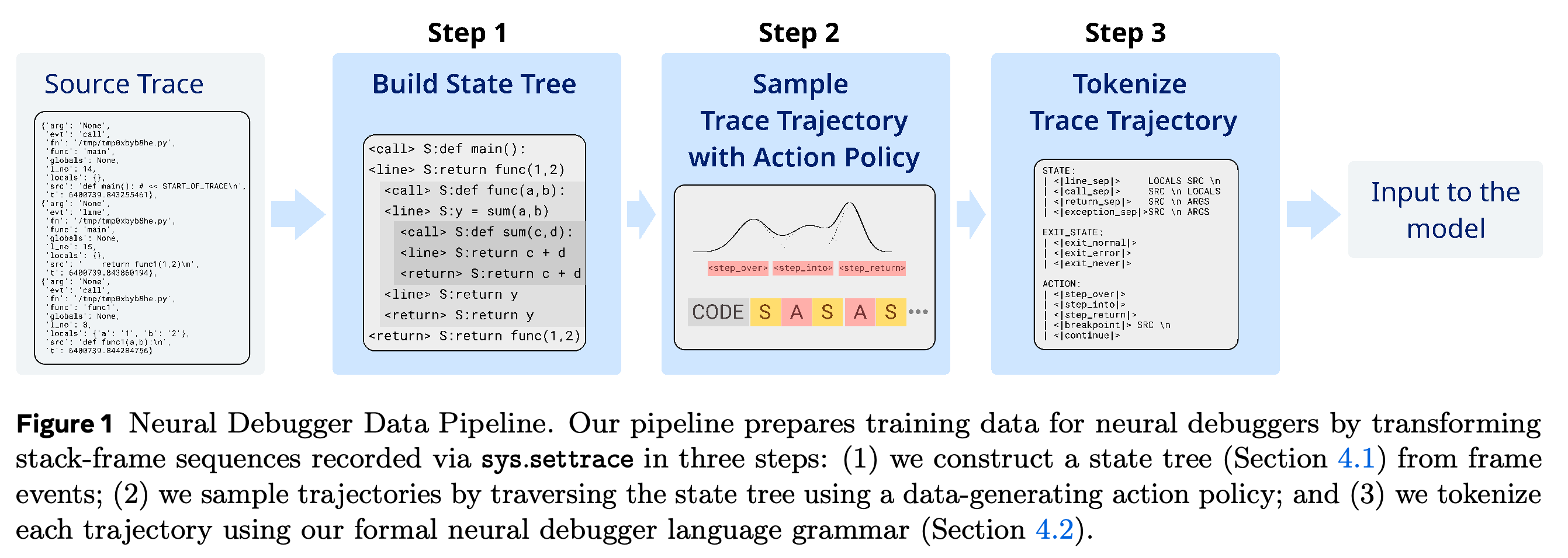
• Figure 1 introduces the three-stage data pipeline: reconstruct a state tree, sample an action-conditioned trajectory, and tokenize the trajectory.

Reconstructing a state tree separates runtime data collection from debugger-specific supervision. Multiple action-conditioned trajectories can then be sampled from an existing execution rather than collecting a separate live debugger session for every action sequence.

2 Related work

Related work includes learned interpreters, scratchpad tracing, dynamic scratchpads, runtime-error prediction, and large-scale execution-trace training. The closest predecessor is CWM, a 32 B-parameter model whose trace format treats executed source lines as actions and variable observations as states.

• CWM can be manually steered during trace generation, but its original format does not directly support jumps to future lines, inverse execution, input inference, or termination prediction.
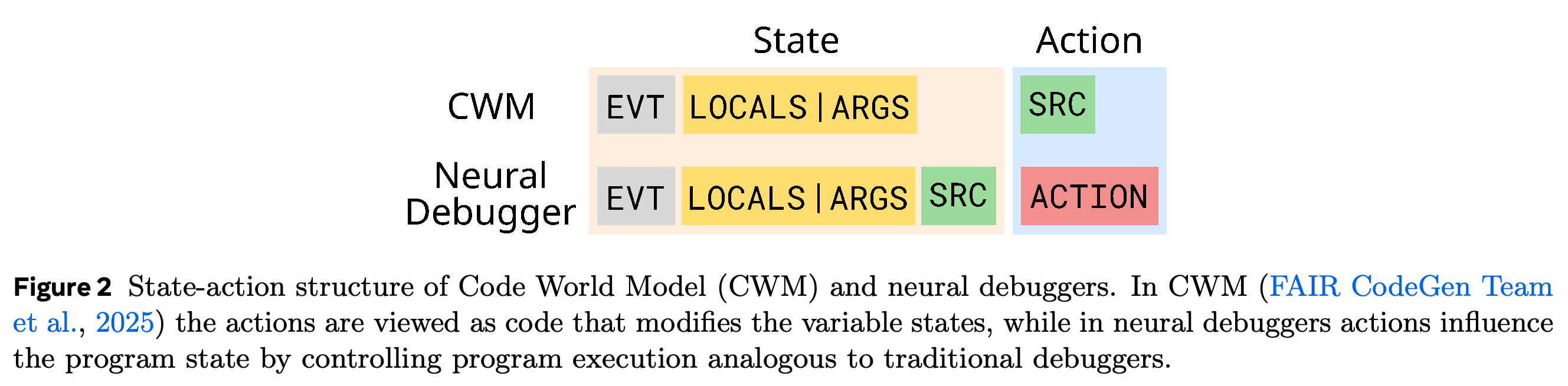
• Figure 2 captures the representational change: the neural debugger includes SRC in the state and uses a separate ACTION field for debugger control.

Moving SRC into the state makes the execution location part of the observation. A separate debugger ACTION requests the transition to predict, replacing CWM’s source-line-as-action representation.

3 Python program execution traces

The dataset records Python execution at the stack-frame level. A custom tracefunc(frame,event,arg), installed through sys.settrace(tracefunc), captures local variables, source lines, runtime event types, and event-specific return or exception arguments while executing functions and repository unit tests.

• Python compiles code blocks into code objects and executes them through stack frames; call and return events provide the information needed to reconstruct nesting.
• The tracing interface is documented at https://docs.python.org/3/library/sys.html#sys.settrace.

4 Neural debugger

A neural debugger is a language model that predicts program execution while accepting symbolic debugger interactions. The method combines an environment formulation, a structured state–action language, and a trajectory-generation pipeline; it learns transition outcomes rather than a policy for choosing useful debugging actions.

4.1 Formulating the debugger as an MDP

The debugger is formulated as an MDP with tuple (S, A, P, R, s0), where S is the program-state space, A contains debugger actions, and s0 denotes possible debugger entry points. The paper defines transitions as P: S × A → S but does not use a reward function, because the training task is state prediction rather than action selection.

• States. Each ordinary program state contains EVT, SRC, and either LOCALS or ARGS, encoding the runtime event, source line, and local values or event-specific arguments. The inverse grammar also includes a synthetic inv_line_call event without a value dictionary.
• Actions. Forward commands are step_into, step_over, step_return, breakpoint SRC, and continue, inspired by conventional debugger interfaces.
• State tree. States belonging to a function call become children of the calling line-event node, preserving execution order while making tree depth correspond to call-stack depth.

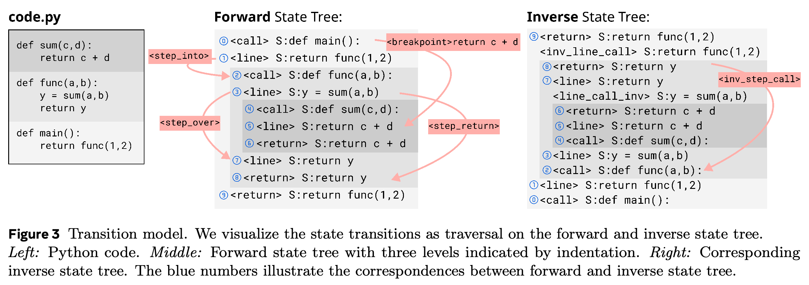
Transitions are explicit traversal rules on the reconstructed state tree, illustrated in Figure 3. Their definitions distinguish entering a nested call from skipping it and distinguish reaching a return event from stopping at a specified source line.

• step_into visits the next recorded state, entering a deeper level when necessary; using only this command recovers the original trace.
• step_over visits the next node at the current level, or moves upward at the level’s end, without descending into a called function.
• step_return reaches the current level’s return-event node. breakpoint SRC reaches the first future occurrence of SRC at any level, or produces the exit code if that line is never reached.
• continue predicts an exit code: normal for regular termination, error for an error or uncaught exception, or never for an infinite loop.

Inverse program execution prediction models plausible predecessors rather than a uniquely determined reversal. Operations such as sorting and addition can map multiple inputs to the same output, so matching one recorded predecessor is not a complete correctness criterion.

• Inverse state tree and inverse transitions. The pipeline reverses state order and duplicates function-calling line nodes as inv_line_call nodes so inverse traversal can enter or skip function calls.
• Inverse breakpoint actions are disabled. inv_step_call replaces step_return and directly predicts a function’s input arguments.
• The model is intended to sample a conditional distribution over predecessor states, unlike a reverse debugger that traverses one fixed history.

The nested example makes the traversal semantics concrete: step_into enters a called function, step_over bypasses its subtree, and step_return targets the current function’s return event. The inverse tree adds call-related nodes so backward navigation can preserve enter-versus-skip choices.

4.2 Formal language for neural debuggers

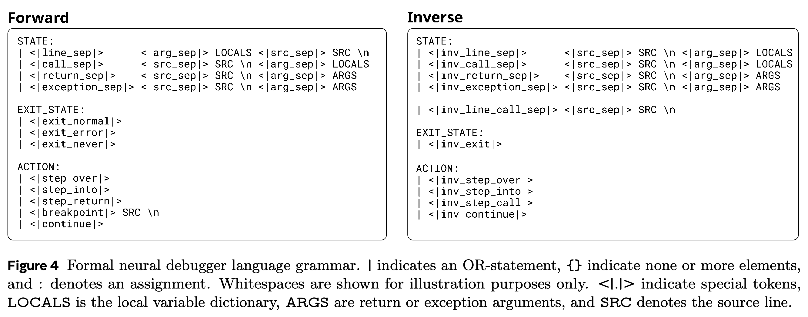
Neural debugger language grammar. A trace contains source-code context followed by state–action pairs and an exit state, with special tokens delimiting each component. Figure 4 specifies separate forward and inverse event and action tokens, extending the CWM representation to encode debugger control.

• Tokens such as <|frame_sep|>, <|action_sep|>, <|src_sep|>, and <|arg_sep|> separate structured observations and commands.
• The inverse grammar includes <|inv_line_call_sep|> and <|inv_step_call|>, while the forward grammar includes <|breakpoint|> followed by SRC.

Distinct event and action tokens let a standard autoregressive language model represent debugger commands and their outcomes. The event schemas also explain component-wise evaluation exclusions: return events carry ARGS rather than LOCALS, and the synthetic inverse call-line event carries only SRC.

Local variable representation. LOCALS is serialized as JSON, with arbitrary Python objects converted to text using __repr__(). Ordinary line transitions show modified variables only and use “..”:”..” to denote omitted unchanged entries.

• Forward trajectories expose all local variables after scope changes, described by the authors as following call, return, or breakpoint events; return-event states themselves carry ARGS in the grammar.
• Inverse traces resolve the complete LOCALS dictionary at call events so all function input variables can be predicted.
• The difference-based format reduces repetition, but text representations of large or complex objects can still dominate trajectory length.

4.3 Debugger trace data pipeline and dataset

Action policy for data generation. A stochastic mixture of categorical action distributions produces trajectories with varied commands while retaining sufficient length. The purpose is to learn action-conditioned transitions, not to imitate expert debugging behavior.

• Data pipeline. Each recorded trace and its visited source-code blocks are transformed into a forward or inverse state tree, sampled into a debugger trajectory, and tokenized with the formal grammar.
• For repository traces, a sampled function call becomes the entry point, restricting the trajectory to that function’s scope.
• Random action and entry-point sampling provide trajectory diversity for repeated training over the underlying execution data.

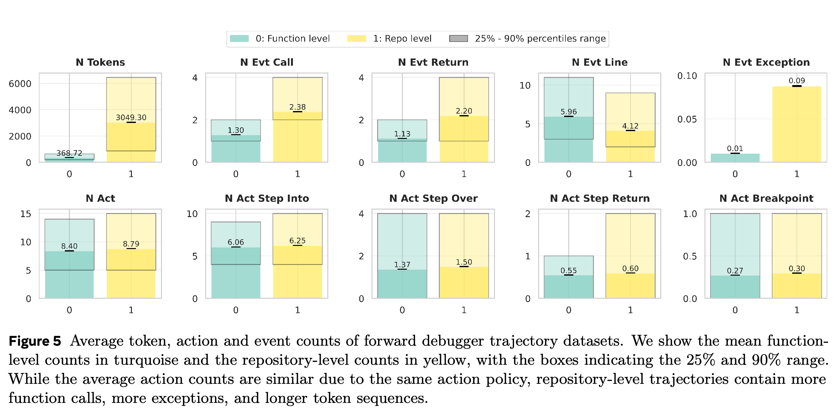
Dataset statistics. Applying the pipeline to CWM execution data yields approximately 15 B repository-level and 100 B function-level debugger trajectory tokens, each total covering forward and inverse directions. Figure 5 shows that repository trajectories have much larger token counts despite similar action counts.

• Mean forward trajectory lengths are 368.72 tokens for function-level data and 3049.30 tokens for repository-level data; mean action counts are 8.40 and 8.79.
• Repository trajectories contain more call, return, and exception events. The authors attribute their larger token counts primarily to larger local dictionaries and more arbitrary Python objects; Appendix A.1 also identifies larger code contexts.

Function-level and repository-level trajectories average 8.40 and 8.79 actions but 368.72 and 3049.30 tokens, respectively. Similar navigation lengths therefore impose substantially different context costs because repository trajectories contain larger observations and more call-related events.

5 Experimental results

Experiment setup. Training uses equal proportions of function-level and repository-level execution traces and includes both forward and inverse directions. The 32 B CWM model is fine-tuned exclusively on debugger data for 50 B tokens, while 1.8 B decoder-only Transformers are pre-trained for 50 B or 150 B tokens.

• Fine-tuning uses linear warmup followed by a constant learning rate; pre-training uses linear warmup followed by cosine decay.
• The smaller models are trained on debugger traces alone or on trace:web:code mixtures of 4:3:1 and 4:6:2, using DCLM web data and GitHub code.
• The evaluations examine full next-state accuracy, accuracy by state component, CruxEval input/output prediction, and sensitivity to prediction horizon.

5.1 Finetuning and pre-training neural debuggers

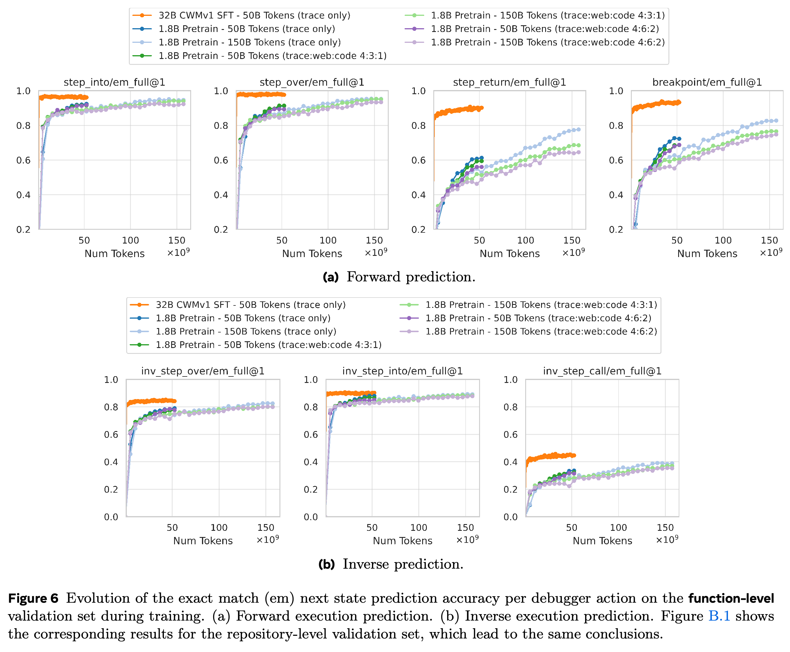
For each debugger action, the authors sample 800 validation trajectories and truncate them after that action to create prediction prompts. Figure 6 reports greedy-decoding exact-match accuracy for complete next states on function-level data; repository-level results are reported separately in the appendix.

• Step actions are easier than jump actions. step_into and step_over plateau earlier and achieve higher accuracy than step_return and breakpoint, which span more intermediate execution states and occur less frequently in the sampled data.
• CWM adapts rapidly to the debugger format, which the authors attribute to its prior exposure to execution traces.
• At 50 B training tokens, the reported large–small model gap is approximately 5 percentage points for step actions and greater than 15 percentage points for jump actions. Training the smaller models for 150 B tokens narrows these gaps, although the comparison also differs in prior training history.

Inverse execution is learnable. Inverse exact-match accuracy improves with training, although it is generally lower than forward accuracy. For inv_step_call, absolute exact-match scores are limited by the possibility of multiple valid inputs, so execution-checked input prediction provides a complementary evaluation.

• Small models are good neural debuggers. The 1.8 B results show that debugger transitions can be learned from scratch, although jump actions remain harder than step actions.
• Mixed-corpus experiments support incorporating debugger traces into web and code training mixtures; they do not measure downstream program-repair benefits.

Step-action curves rise and saturate sooner than jump-action curves, while longer training particularly benefits the smaller models on jumps. The low inv_step_call exact-match values measure agreement with recorded inputs, not the rate of all execution-valid input predictions.

5.2 Next program state prediction by state component

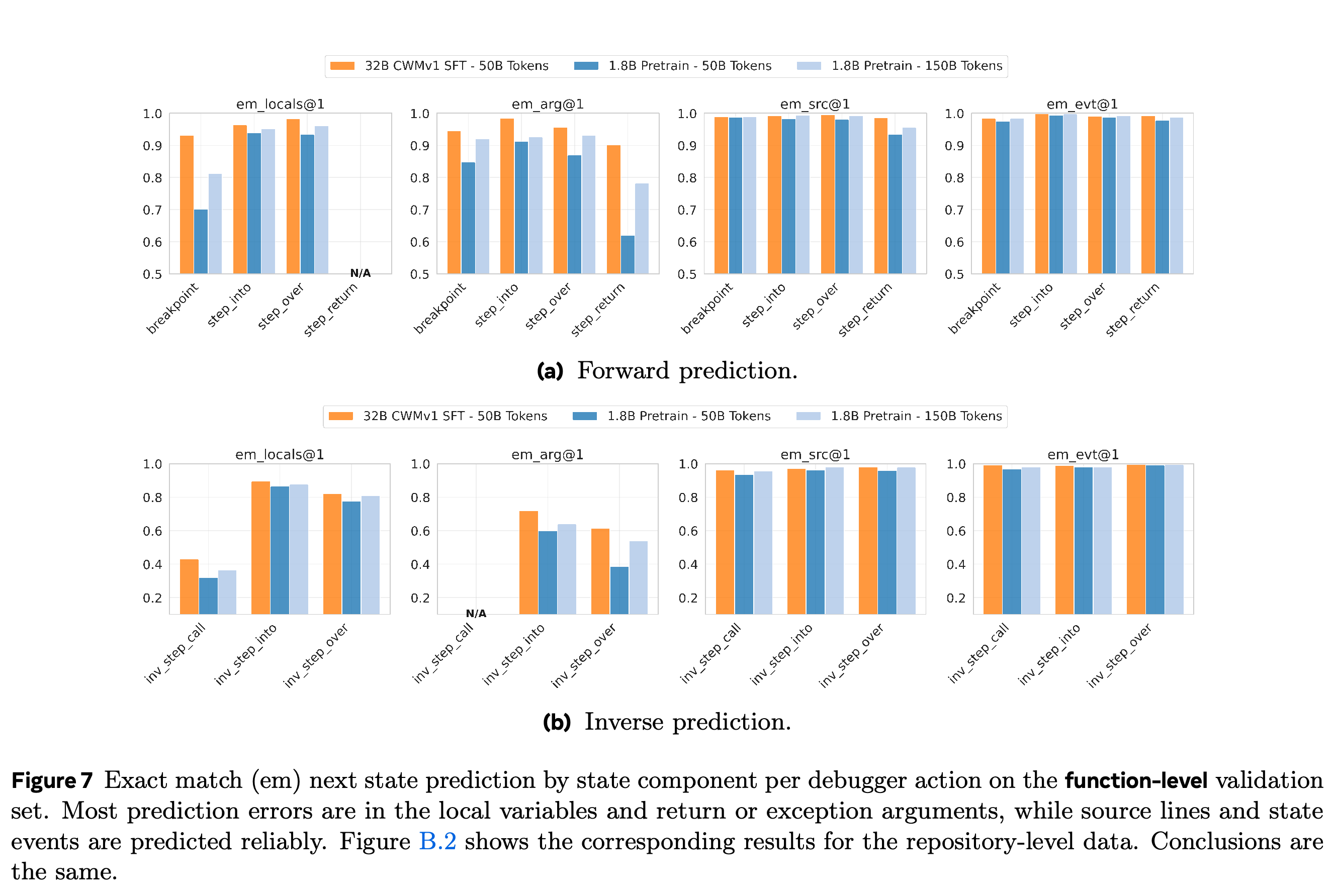
Source lines & state events are predicted reliably; local variables contain errors. Figure 7 decomposes exact-match accuracy into LOCALS, ARGS, SRC, and EVT for models trained exclusively on debugger traces. Most residual errors and most large–small model gaps arise in local values and return or exception arguments rather than source-line or event prediction.

• For the 1.8 B models, step_return source-line accuracy exhibits a reported drop of approximately 5 percentage points on function-level data and 10 percentage points on repository-level data; the authors hypothesize that repository code has more complex conditional branching.
• N/A denotes a state component absent from a particular target event, not an unsuccessful prediction.
• inv_step_call local-dictionary exact match measures agreement with one recorded input and does not account for alternative valid predecessors.

SRC and EVT accuracy remains high across most actions, whereas LOCALS and ARGS show larger errors and model-size gaps. This decomposition identifies value prediction as the principal remaining difficulty, with inverse input ambiguity additionally depressing inv_step_call local-dictionary exact match.

5.3 Input and output prediction on CruxEval

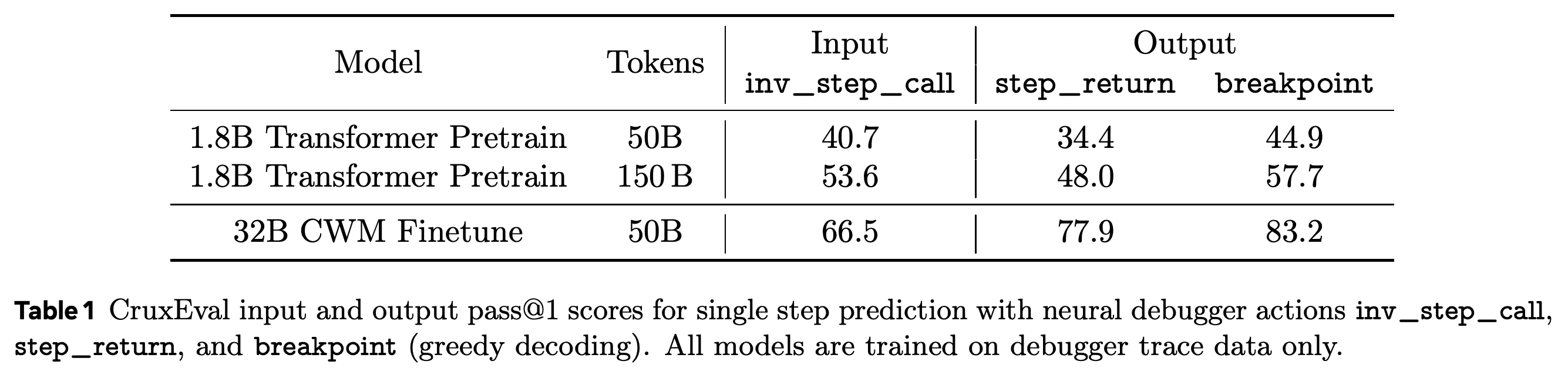
CruxEval tasks are expressed as debugger jumps: inv_step_call predicts inputs, while step_return and breakpoint predict outputs. Table 1 uses greedy decoding and execution-based pass@1, checking predicted inputs with assert f(predicted_input) == reference_output rather than requiring the reference input itself.

• The trace-only 1.8 B model trained for 50 B tokens scores 40.7 for inputs, 34.4 for step_return outputs, and 44.9 for breakpoint outputs.
• At 150 B tokens, its corresponding scores are 53.6, 48.0, and 57.7; the fine-tuned 32 B CWM scores 66.5, 77.9, and 83.2.
• Neural debuggers excel at output prediction. The 77.9 step_return score exceeds the cited stock-CWM trace-step result of 58.1 by 19.8 percentage points.

breakpoint performs better than step_return, which the authors attribute to its prompt explicitly supplying the return statement’s source line. This reduces the need to identify the target execution location, so the two output scores reflect different conditioning information.

• A step_return target contains a return event and its argument; a breakpoint target contains the local dictionary at the specified return line.
• The appendix provides concrete examples of both output prompts and the inverse input prompt.

The fine-tuned 32 B model scores 66.5 for input prediction and 77.9 or 83.2 for output prediction, depending on the action. The consistent breakpoint advantage must be interpreted alongside its explicit return-line prompt; input pass@1 accepts alternative inputs when executing them produces the required output.

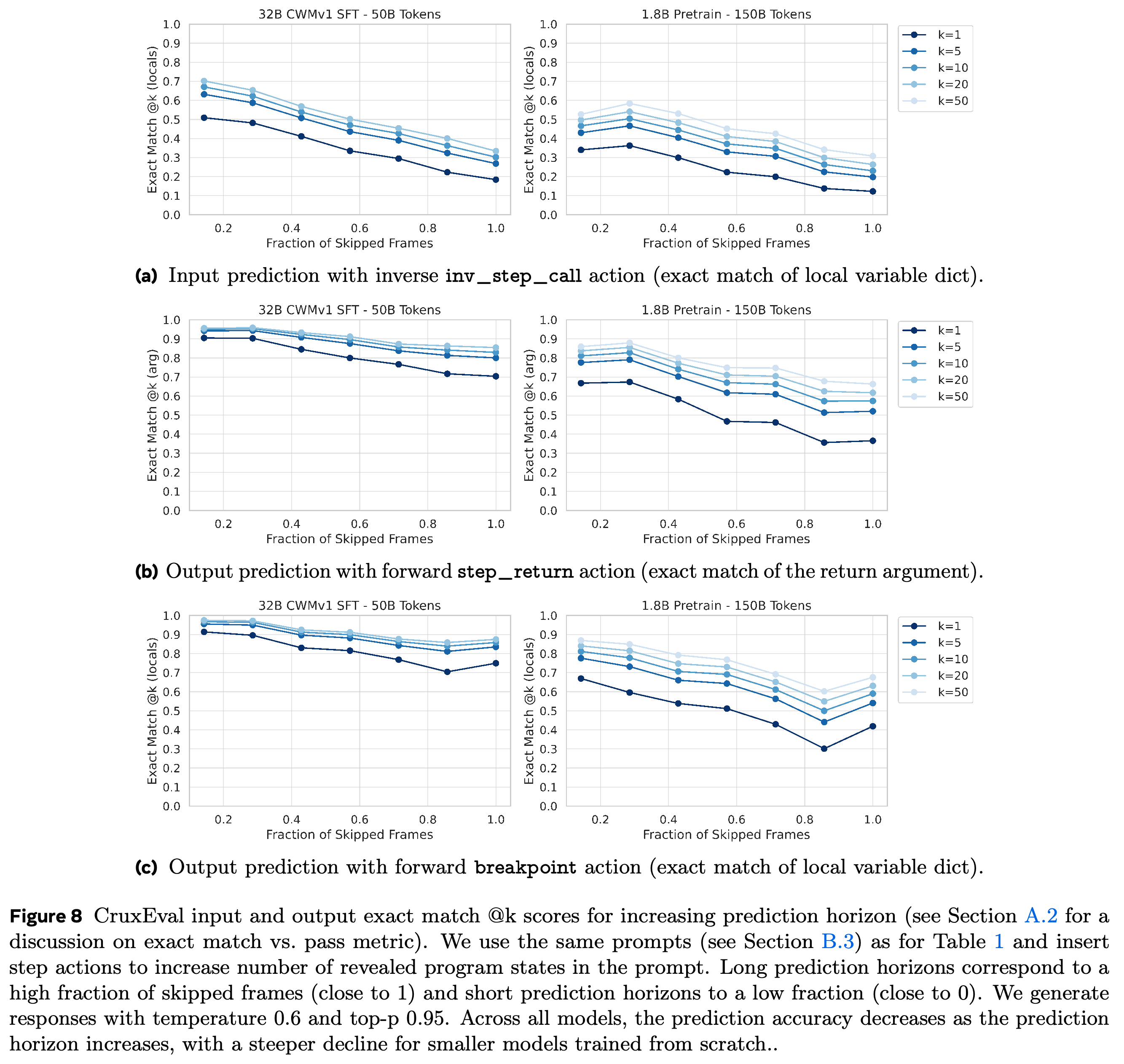
Prediction accuracy decreases with prediction horizon. Figure 8 varies the fraction of intermediate frames skipped before the final jump and reports exact match @k for k = 1, 5, 10, 20, and 50, using temperature 0.6 and top-p 0.95. The curves show an overall decline rather than a strictly monotonic decrease in every panel.

• A skipped-frame fraction near 0 represents a short transition, while a fraction near 1 represents prediction across the full function.
• Accuracy generally falls with longer horizons, with larger declines for the 1.8 B model. Larger sampling budgets partially reduce the loss.
• Input and breakpoint curves measure reference local-dictionary exact match, while step_return curves measure return-argument exact match. Unlike Table 1, this evaluation uses stochastic decoding; ensembling, uncertainty-guided resampling, and adaptive jump selection are proposed extensions, not tested methods.

Increasing the skipped-frame fraction generally reduces accuracy, especially for the smaller model, while additional samples recover some accuracy. The trend is not strictly monotonic in every panel. Input and breakpoint panels evaluate local-dictionary exact match, and stochastic decoding further distinguishes these curves from Table 1’s greedy execution-checked scores.

6 Limitations and future work

The demonstrated downstream application is input/output prediction, not automated repair. Agentic program repair, reasoning & tool use with neural debuggers remains future work, including self-debugging generated code and controlling real debugging tools.

• Expanding & improving data generation. The study covers Python and random action policies; the authors propose additional languages and syntax-aware or goal-directed trajectory sampling.
• Improving inverse debugging. Better modeling of feasible value sets and evaluation across multiple valid predecessors are needed to handle ambiguous inverse states.
• Better Python object representations. __repr__()-based serialization becomes impractical for very large or complex structures, particularly in repository-level traces.

7 Conclusion

The paper introduces an action-conditioned execution-modeling interface and a trace-to-trajectory pipeline, then shows that fine-tuned large models and smaller models trained from scratch can learn debugger transitions. Intermediate-state and CruxEval results support execution-prediction capabilities; using these models as world models for coding agents remains an untested extension.

Appendix

• A Extended neural debugger and A.1 Extended debugger trace dataset provide trajectory-length histograms and the action-policy mixture. Table A.1 selects each of two policies with probability 0.5: the displayed first row assigns step_into, step_over, step_return, breakpoint, and continue probabilities of 0.35, 0.1, 0.2, 0.1, and 0.05; the second assigns 0.5 each to step_into and step_over. The first displayed row sums to 0.8 and is nonuniform, despite the accompanying prose describing uniform sampling, leaving an unresolved specification inconsistency.
• A.2 Evaluating Inverse Execution Prediction distinguishes matching a reference input from producing any input that executes to the required output. Table A.2 reports input exact_match@1 versus pass@1 of 14.3 versus 40.7 for the 1.8 B/50 B-token model, 17.7 versus 53.6 for the 1.8 B/150 B-token model, and 23.1 versus 66.5 for fine-tuned CWM. These gaps demonstrate that single-reference exact match understates execution-valid input prediction; the authors propose dedicated execution-based evaluations for broader debugger capabilities.
• B Extended experiments and B.1 Training recipe specify AdamW with weight decay 0.1 and a Llama-2 architecture for the 1.8 B models. Both training regimes use 750 warmup steps; pre-training peaks at 1 × 10−3 and decays to zero, while fine-tuning peaks at 1 × 10−5 and remains constant. All experiments use sequence length 16 384 and batch size 1 M tokens or 64 sequences.
• B.2 Extended next state prediction results repeats the main action-wise and component-wise analyses on repository-level validation data, with similar qualitative conclusions. B.3 CruxEval input and output prediction prompts in neural debugger format shows how step_return predicts a return argument, breakpoint predicts locals at the return line, and inv_step_call predicts function arguments. C Neural debugger trace example follows count(“berry”, “r”) forward to output 2 and illustrates an inverse trajectory, while noting infinitely many possible s and t combinations yielding n=2.

Brief Thoughts

The central contribution is the execution-model interface: debugger actions select which transition the model must predict instead of requiring every intermediate line. The state-tree construction defines these transitions precisely, and the component-wise results indicate that predicting control-flow locations is easier than predicting the values exposed at those locations.

The execution-checked CruxEval evaluation and the gap between inverse exact match and pass@1 provide the clearest evidence for useful conditional execution modeling. Practical debugging utility remains uncertain because repair and bug localization are not evaluated, breakpoint prompts provide extra target-location information, and long-horizon value prediction remains error-prone.