Gorio Tech Blog search

GTN(Graph Transformer Networks) 설명

|

이번 글에서는 GTN이란 알고리즘에 대해 다뤄보겠다. 상세한 내용은 논문 원본을 참고하길 바라며, 본 글에서는 핵심적인 부분에 대해 요약 정리하도록 할 것이다. 저자의 Gitub에서 코드를 참고할 수도 있다.


Graph Transformer Networks 설명

1. Introduction

대다수의 GNN 연구가 fixed & homogenous graph에 대한 것인 반면, GTN은 다양한 edge와 node type을 가진 heterogenous graph에 대한 효과적인 접근을 위해 고안되었다. heterogenous graph 혹은 relational graph에 대한 연구의 대표적인 예시라고 하면 RGCN을 들 수 있겠는데, GTNRGCN과는 다른 방식으로 여러 edge(relation) type을 핸들링한다. 다만 논문에서는 여러 node type에 대해서 분명한 언급을 하고 있지는 않다.

어쨌든 GTN은 모델이 type 정보를 활용하지 못함으로써 suboptimal한 결과를 얻는 것을 방지하기 위해 학습을 통해 복수의 meta-path를 생성하여 다시 한 번 heterogenous graph를 재정의하는 과정을 거치게 된다. 그리고 이후 downstream task에 맞게 GNN layer (논문에서는 classic GCN을 사용)를 붙여서 모델의 구조를 완성한다.


2. Meta-Path Generation

GTN에서의 meta-path는 heterogenous graph에서 여러 edge(relation) type을 부드럽게 조합한 새로운 graph 구조를 생성하는 과정으로 정의할 수 있다.

$t_1, t_2, …, t_l$ 의 edge type이 존재한다고 할 때, 이 특정 edge type에 맞는 인접 행렬은 $A_{t_1}, A_{t_2}, …, A_{t_l}$ 이라고 표현할 수 있다. 이 때 meta-path $P$ 의 인접 행렬은 이들의 행렬 곱으로 이루어진다.

[A_P = A_{t_1} A_{t_2} … A_{t_l}]

예를 들어 Author-Paper-Conference 라는 meta-path가 있다고 하자. 그렇다면 이는 아래와 같이 표현할 수 있다.

[A \xrightarrow{AP} P \xrightarrow{PC} C]

이 meta-path $APC$ 의 인접 행렬은 $A_{APC} = A_{AP} A_{PC}$ 이다.

그렇다면 실제 GTN에서는 meta-path를 어떻게 생성할까.

$K$ 개의 edge type이 존재하는 heterogenous graph가 존재할 때, 각 edge type을 분리하여 인접 행렬을 생성한 뒤 이를 겹쳐 놓으면 $\mathbb{A} = (N, N, K)$ 를 구성할 수 있다.

이 때 weight에 softmax 함수를 적용하고 out_channels의 수를 $C$ 개로 설정한 1x1 Convolution 을 적용하면 이 인접 행렬은 $(N, N, C)$ 의 형상을 갖게 된다. 즉 기존의 $K$ 개의 edge type 들이 새로운 방식으로 조합되어 $C$ 개의 relation을 구성하게 된 것이다.

이렇게 2개의 결과를 만들어 낸 것이 $Q_1^1, Q_2^1$ 이고, 이들은 Selected Adjacency Matrices라고 부른다. 즉, 2번에 걸쳐 meta-path를 생성한 것이라고 볼 수 있다. 다시 이들을 곱한 뒤 normalization을 적용해주면 1번째 meta-path 인접 행렬인 $A^1$ 을 얻을 수 있다.

[A^1 = D^{-1} Q_1^1 Q_2^1]

그리고 짧은/긴 meta-path를 모두 성공적으로 학습하기 위해 $\mathbf{A} = \mathbf{A} + I$ 작업은 추가해준다.

한 번 더 $Q$ 를 만들어 내면 이를 $Q^2$ 라고 명명하고, 이전 결과인 $A^1$ 과 곱하여 $A^2$ 를 생성하게 된다. $l$ 번째로 $Q$ 를 만들어 내면 이 행렬은 $Q^l$ 이 되고, 이전 결과인 $A^{l-1}$ 과 곱하여 최종 결과인 $A^l$ 을 얻게 된다.


3. Graph Transformer Networks

$l$ 개의 graph transformer layer를 이용했다면 현재 결과인 composite adjacency matrix $A^l$ 은 총 $C$ 개의 새로운 relation에 대한 정보를 포함하고 있을 것이다. 이제 이 행렬을 다시 $C$ 개의 2D 행렬로 분해한 후, 각각에 대해 GNN을 적용한 뒤 concatenation operator를 통해 최종 결과인 $Z$ 행렬을 얻는다.

[Z = \mathbin\Vert_{i=1}^C \sigma ( \tilde{D}_i^{-1} \tilde{A}_i^l X W )]

[= [\tilde{D}_1^{-1} \tilde{A}_1^l X W, \tilde{D}_2^{-1} \tilde{A}_2^l X W, …]]

이 때 $\tilde{D}_i^{-1}, \tilde{A}_i^l$ 는 $(N, N)$, $X$ 는 $(N, d)$, $W$ 는 $(d, d)$ 의 shape을 가진다. 그리고 $W$ 의 경우 모든 channel(new relation)에 대하여 공유되는 trainable parameter이다.


4. Conclusion

실험 결과에 대해서는 논문 원본을 참조하길 바란다.

몇 가지 사항을 정리하면서 글을 마무리한다.

1) 1x1 Convolution layer의 weight는 softmax 함수를 적용하여 meta-path를 생성할 때 candidate 인접 행렬에 대한 attention score의 역할을 수행한다. 이를 통해 각 edge(relation) type에 대한 중요도를 가늠해 볼 수 있다.

2) 본 논문에서는 classic GCN을 사용하였지만 task에 따라 다른 GNN layer를 붙여볼 수 있을 것이다. 흥미로운 layer 구성이 많으므로 여러 응용 버전을 기대해 볼 수 있다.

3) GTN은 Full-training에 기반하여 설계되었기 때문에 규모가 큰 graph에 대해서는 수정된 접근이 필요할 것으로 보인다.

4) 본 논문에서는 Embedding Size는 64를 사용하였고, 데이터셋에 따라 다르지만 graph transformer layer는 2~3개 정도를 사용하였다. 데이터셋의 크기가 크지 않아 $C$ 의 크기나 layer의 수 모두 작게 설정하였는데, task에 따라 tuning이 필요할 것으로 보인다.

Comment  Read more

Pytorch Geometric custom graph convolutional layer 생성하기

|

Pytorch GeometricMessagePassing class에 대한 간략한 설명을 참고하고 싶다면 이 글을 확인하길 바란다.

본 글에서는 MessagePassing class를 상속받아 직접 Graph Convolutional Layer를 만드는 법에 대해서 다루도록 하겠다. 그 대상은 RGCN: Relational GCN이다. RGCN에 대한 간략한 설명을 참고하고 싶다면 이 곳을 확인해도 좋고 RGCN source code를 확인해도 좋다.


Custom GCN layer 생성하기: RGCN

본 포스팅에서는 원본 source code의 형식을 대부분 보존하면서도 간단한 설명을 위해 필수적인 부분만 선별하여 설명의 대상으로 삼도록 할 것이다.

먼저 필요한 library를 불러오고 parameter를 초기화하기 위한 함수를 선언한다.

import math
from typing import Optional, Union, Tuple

from torch.nn import Parameter

from torch_geometric.typing import OptTensor, Adj
from torch_geometric.nn.conv import MessagePassing

def glorot(tensor):
    if tensor is not None:
        stdv = math.sqrt(6.0 / (tensor.size(-2) + tensor.size(-1)))
        tensor.data.uniform_(-stdv, stdv)

def zeros(tensor):
    if tensor is not None:
        tensor.data.fill_(0)        

RGCN에서는 regularization 방법으로 2가지를 제시하고 있는데 본 포스팅에서는 자주 사용되는 basis-decomposition 방법을 기본으로 하여 진행하도록 하겠다.

예를 들기 위해 적합한 데이터를 생각해보자. (참고로 아래 setting은 MUTAG 데이터셋을 불러온 것이다. 아래 코드를 통해 다운로드 받을 수 있다.)

dataset = 'MUTAG'

path = os.path.join(os.getcwd(), 'data', 'Entities')
dataset = Entities(path, dataset)
data = dataset[0]
구분 설명
edge_index (2, 148454)
edge_type (148454), 종류는 46개
num_nodes 23606
x node features는 주어지지 않음

그렇다면 이 layer의 목적은 23606개의 node에 대하여, 46종류의 relation을 갖는 edges를 통해 message passing을 진행하는 것이다. MUTAG 데이터셋에는 node features는 존재하지 않지만, data.x = torch.rand((23606, 100)) 코드를 통해 가상의 데이터를 만들어서 임시로 연산 과정을 살펴볼 수 있을 것이다.

먼저 반드시 필요한 사항에 대해 정의해보자.

class RelationalGCNConv(MessagePassing):
    def __init__(self,
                 in_channels: int,
                 out_channels: int,
                 num_relations: int,
                 num_bases: Optional[int]=None,
                 aggr: str='mean',
                 **kwargs):
        super(RelationalGCNConv, self).__init__(aggr=aggr, node_dim=0)

        # aggr, node_dim은 알아서 self의 attribute로 등록해준다. (MessagePassing)
        self.in_channels = in_channels
        self.out_channels = out_channels
        self.num_relations = num_relations
        self.num_bases = num_bases

        # 원본 코드에서 in_channels가 tuple인 이유는
        # src/tgt node가 다른 type인 bipartite graph 구조도 지원하기 위함이다.
        # 예시를 위해 integer로 변경한다.
        self.in_channels = in_channels

RGCN은 Full-batch training을 기본으로 하고 있다. 이 때문에 node_dim을 조정해 주어야 한다.

다음으로는 Weight Parameter를 정의해주자. 이해를 쉽게 하기 위해서 원본 코드에서 변수 명을 수정하였다.

        # Define Weights
        if num_bases is not None:
            self.V = Parameter(
                data=Tensor(num_bases, in_channels, out_channels))
            self.a = Parameter(Tensor(num_relations, num_bases))
        else:
            self.V = Parameter(
                Tensor(num_relations, in_channels, out_channels))
            # dummy parameter
            self.register_parameter(name='a', param=None)

        self.root = Parameter(Tensor(in_channels, out_channels))
        self.bias = Parameter(Tensor(out_channels))

        self.reset_parameters()

basis-decomposition의 식을 다시 확인해보자.

[W_r^l = \Sigma_{b=1}^B a_{rb}^l V_b^l]

reset_parameters 메서드는 아래와 같다.

    def reset_parameters(self):
        glorot(self.V)
        glorot(self.a)
        glorot(self.root)
        zeros(self.bias)

이제 본격적으로 forward 함수를 구현할 차례이다. 사실 RGCN의 경우 특별히 변형을 하지 않느다면, 특정 relation 안에서의 연산은 일반적인 GCN과 동일하다. 따라서 기본적 세팅에서는 message, aggregate, update 메서드를 override할 필요가 없다.

다음은 forward 함수의 윗 부분이다.

    def forward(self,
                x: OptTensor,
                edge_index: Adj,
                edge_type: OptTensor=None):

        x_l = x
        # node feature가 주어지지 않는다면
        # embedding weight(V) lookup을 위해 아래와 같이 세팅한다.
        if x_l is None:
            x_l = torch.arange(self.in_channels, device=self.V.device)

        x_r = x_l
        size = (x_l.size(0), x_r.size(0))

        # output = (num_nodes, out_channels)
        out = torch.zeros(x_r.size(0), self.out_channels, device=x_r.device)

num_bases 인자가 주어진다면 아래와 같이 weight를 다시 계산해준다.

        V = self.V
        if self.num_bases is not None:
            V = torch.einsum("rb,bio->rio", self.a, V)

자 이제 각 relation 별로 propagate를 진행해주면 된다. 앞서 언급하였듯이 특정 relation 내에서의 연산은 일반적인 GCN과 다를 것이 없다. 참고로 아래와 같이 계산하면 속도 측면에서 매우 불리한데, 이를 개선한 FastRGCNConv layer가 존재하니 참고하면 좋을 것이다. 다만 이 layer의 경우 메모리를 크게 사용하므로 본격적인 사용에 앞서 점검이 필요할 것이다.

        # propagate given relations
        for i in range(self.num_relations):
            # 특정 edge_type에 맞는 edge_index를 선별한다.
            selected_edge_index = masked_edge_index(edge_index, edge_type == i)

            # node_features가 주어지지 않는다면
            if x_l.dtype == torch.long:
                out += self.propagate(selected_edge_index, x=V[i, x_l], size=size)

            # node_features가 주어진다면
            else:
                h = self.propagate(selected_edge_index, x=x_l, size=size)
                out += (h @ V[i])

        out += self.root[x_r] if x_r.dtype == torch.long else x_r @ self.root
        out += self.bias
        return out

masked_edge_index 함수는 아래와 같다.

from torch_sparse import masked_select_nnz

def masked_edge_index(edge_index, edge_mask):
    """
    :param edge_index: (2, num_edges)
    :param edge_mask: (num_edges) -- source node 기준임
    :return: masked edge_index (edge_mask에 해당하는 Tensor만 가져옴)
    """
    if isinstance(edge_index, Tensor):
        return edge_index[:, edge_mask]
    else:
        # if edge_index == SparseTensor
        return masked_select_nnz(edge_index, edge_mask, layout='coo')

여기까지 진행했다면 custom gcn layer 구현은 끝난 것이다. 아래와 같이 사용하면 된다.

data = data.to(device)

model = RelationalGCNConv(
    in_channels=in_channels, out_channels=out_channels,
    num_relations=num_relations, num_bases=num_bases).to(device)

print(get_num_params(model))

out = model(x=data.x, edge_index=data.edge_index, edge_type=data.edge_type)
Comment  Read more

MMDetection 사용법 2(Tutorial)

|

이 글에서는 MMDetection를 사용하는 방법을 정리한다.

이전 글에서는 설치 및 Quick Run 부분을 다루었으니 참고하면 좋다.


Tutorial 1: Learn about Configs

이미 만들어져 있는 모델이나 표준 데이터셋만을 활용하고자 한다면, config 파일만 적당히 바꿔주면 다른 건 할 것 없이 바로 코드를 돌려볼 수 있다.

먼저 config 파일의 구조는 다음과 같다.

  • 기본이 되는 config 파일이 configs/_base_/ 디렉토리에 있다. 해당 디렉토리는 dataset, model, schedule, default_runtime 총 4개로 구성되며 사용되는 config들은 이들을 base로 한다. _base_ 안에 있는 config로만 구성된 config를 primitive라 한다.
  • 실제로 사용할 config는 _base_ 내의 기본 config 또는 다른 config를 상속받아 구성할 수 있다. 이를테면 하나의 primitive를 상속받은 뒤 적당한 수정을 가해서 사용하는 방식이다.
    • 만약 아예 새로운 config를 만들고 싶다면 configs/에다 새로운 디렉토리를 만들고 작성하면 된다.

config 디렉토리의 구조는 대략 다음과 같음을 기억하자.

mmdetection
├── configs
│   ├── _base_
│   │   ├── datasets
|   │   │   ├── coco_detection.py
|   │   │   ├── ...
│   │   ├── models
|   │   │   ├── faster_rcnn_r50_fpn.py
|   │   │   ├── ...
│   │   ├── schedules
|   │   │   ├── schedule_1x.py
|   │   │   ├── ...
│   │   ├── default_runtime.py
|   |
│   ├── faster_rcnn
|   │   ├── faster_rcnn_r50_fpn_1x_coco.py
|   │   ├── ...
│   ├── mask_rcnn
│   ├── ...

primitive의 한 예시는 configs/faster_rcnn/faster_rcnn_r50_fpn_1x_coco.py이다.

_base_ = [
    '../_base_/models/faster_rcnn_r50_fpn.py',
    '../_base_/datasets/coco_detection.py',
    '../_base_/schedules/schedule_1x.py', '../_base_/default_runtime.py'
]

이미 만들어진 위의 config configs/faster_rcnn/faster_rcnn_r50_fpn_1x_coco.py에다가 약간의 수정을 가한 config의 예시는 configs/faster_rcnn/faster_rcnn_r50_fpn_bounded_iou_1x_coco.py이다.

_base_ = './faster_rcnn_r50_fpn_1x_coco.py'
model = dict(
    roi_head=dict(
        bbox_head=dict(
            reg_decoded_bbox=True,
            loss_bbox=dict(type='BoundedIoULoss', loss_weight=10.0))))

이 config는 BoundedIoULoss를 사용하는 것을 제외하면 faster_rcnn_r50_fpn_1x_coco와 완전히 같은 모델이다. _base_에서 모든 설정을 가져온 뒤, 아래에 있는 부분만 덮어씌워진다.
이처럼 이미 있는 모델 config에다가 약간만 수정해서 갖다쓰면 되는 간단한 방식이다.

참고로 tools/train.pytools/test.py를 실행시킬 때 --cfg-options 옵션으로 추가로 지정할 수 있다.


config 작명 방법

이름이 faster_rcnn_r50_fpn_1x_coco와 같이 꽤 긴 것을 볼 수 있다. 많은 정보를 담고 있는데, 일반적인 형식은 다음과 같다.

{model}_[model setting]_{backbone}_{neck}_[norm setting]_[misc]_[gpu x batch_per_gpu]_{schedule}_{dataset}

{중괄호}는 필수, [대괄호]는 선택이다.

  • {model}: faster_rcnn와 같은 모델 이름이다.
  • {model setting}: 일부 모델에 대한 세부 설정인데 htc의 경우 without_semantic, reppoints의 경우 moment 등이다.
  • {backbone}: 모델의 전신이 되는 기본 모델로 r50(ResNet-50), x101(ResNeXt-101) 등이다.
  • {neck}: 모델의 neck에 해당하는 부분을 정하는 것으로 fpn, pafpn, nasfpn, c4 등이 있다.
  • {norm_setting}: 기본값은 bn으로 batch normalization이며 생략이 가능하다. gn은 Group Normalization, syncbn은 Synchronized BN, gn-headgn-neck은 GN을 head 또는 neck에만 적용, gn-all은 모델의 전체(backbone, nect, head)에다가 GN을 적용한다.
  • [misc]: 이모저모를 적자. dconv, gcb, attention, albu, mstrain 등이다.
  • [gpu x batch_per_gpu]: GPU 개수와 GPU 당 sample 개수로 8x2가 기본이다.
  • {schedule}: 1x는 12epoch, 2x는 24epoch이며 8/16번째와 11/22번째 epoch에서 lr이 10분의 1이 된다. 20e는 cascade 모델에서 사용되는 것으로 20epoch으로 10분의 1이 되는 시점은 16/19번째이다.
  • {dataset}: 데이터셋을 나타내는 부분으로 coco, cityscapes, voc_0712, wider_face 등이다.

config 파일 예시

_base_ 내의 Faster R-CNN config 파일은 다음과 같이 생겼다.

# model settings
model = dict(
    type='FasterRCNN',
    pretrained='torchvision://resnet50',
    backbone=dict(
        type='ResNet',
        depth=50,
        num_stages=4,
        out_indices=(0, 1, 2, 3),
        frozen_stages=1,
        norm_cfg=dict(type='BN', requires_grad=True),
        norm_eval=True,
        style='pytorch'),
    neck=dict(
        type='FPN',
        in_channels=[256, 512, 1024, 2048],
        out_channels=256,
        num_outs=5),
    rpn_head=dict(
        type='RPNHead',
        ...
        ),
    roi_head=dict(
        type='StandardRoIHead',
        ...
        ),
    # model training and testing settings
    train_cfg=dict(
        rpn=dict(...),
        rpn_proposal=dict(...),
        rcnn=dict(...),
    test_cfg=dict(
        rpn=dict...),
        rcnn=dict(...)
        # soft-nms is also supported for rcnn testing
        # e.g., nms=dict(type='soft_nms', iou_threshold=0.5, min_score=0.05)
    ))

대충 살펴보면,

  • type: Faster RCNN 모델이다.
  • pretrained: torchvision의 pretrained model 중 resnet50을 가져온다.
  • backbone: backbone 모델의 세부를 결정하는데, 이 경우 50 layer짜리 resnet으로 BN을 사용한다.
  • neck: backbone 모델과 head를 잇는 부분이다. 여기서는 FPN을 사용하였으며 채널 수 등이 정의되어 있다.
  • head: rpn headroi head가 사용된다.
  • train_cfg, test_cfg: iou threshold, 이미지 개수 등 세부를 조절한다. 참고로 위의 코드처럼 model config안에 넣어야 한다. config file 제일 바깥에 쓰는 방법은 deprecated된 상태이다.

Tutorial 2: Customize Datasets

표준 데이터셋 이외에 다른 데이터셋을 사용하려면 먼저 COCO format이나 middle format으로 변환해야 한다.

추천하는 방법은 학습 중에 하는(online) 방법 대신 미리(offline) COCO format으로 변환하는 것이라고 한다.

COCO format으로 변환

COCO 기준 데이터는 다음과 같이 구성하면 된다.

mmdetection
├── configs
├── data
│   ├── coco
│   │   ├── annotations
|   │   │   ├── captions_train2017.json
|   │   │   ├── ...
│   │   ├── train2017
|   │   │   ├── 000000000009.jpg
|   │   │   ├── ...
│   │   ├── val2017
|   │   │   ├── 000000000139.jpg
|   │   │   ├── ...
│   │   ├── test2017
|   │   │   ├── 000000000001.jpg
|   │   │   ├── ...
...

annotation 형식이 중요한데, COCO format은 다음과 같다.

'images': [
    {
        'file_name': 'COCO_val2014_000000001268.jpg',
        'height': 427,
        'width': 640,
        'id': 1268
    },
    ...
],

'annotations': [
    {
        'segmentation': [[192.81,
            247.09,
            ...
            219.03,
            249.06]],  # if you have mask labels
        'area': 1035.749,
        'iscrowd': 0,
        'image_id': 1268,
        'bbox': [192.81, 224.8, 74.73, 33.43],
        'category_id': 16,
        'id': 42986
    },
    ...
],

'categories': [
    {'id': 0, 'name': 'car'},
    ...
]

필수로 포함되어야 하는 부분은 다음 3가지다.

  • images: 이미지 파일에 대한 기본정보를 나타내는 list로 file_name, height, width, id 등이 들어간다.
  • annotations: 각 이미지 파일에 대한 annotation 정보의 list이다.
  • categories: 카테고리 name과 그 id가 포함된 list 형태이다.

각 부분 내에서 세부적인 내용은 조금씩 다를 수 있다.

Customized dataset 사용을 위한 config 파일 수정

사용자 지정 config 파일을 configs/my_custom_config.py라 하면 다음 두 부분을 수정해야 한다.

  1. data.train, data.val, data.test에 있는 classes에 명시적으로 추가해야 한다.
  2. model 부분에서 num_classes를 덮어씌운다. COCO는 80으로 되어 있다. 데이터셋마다 class의 개수가 다를 텐데 이를 지정해야 한다.

뭐 다음과 같은 식이다. base인 cascade_mask_rcnn_r50_fpn_1x_coco에다가 데이터셋 정보만 업데이트한 것이다.

# the new config inherits the base configs to highlight the necessary modification
_base_ = './cascade_mask_rcnn_r50_fpn_1x_coco.py'

# 1. dataset settings
dataset_type = 'CocoDataset'
classes = ('a', 'b', 'c', 'd', 'e')
data = dict(
    samples_per_gpu=2,
    workers_per_gpu=2,
    train=dict(
        type=dataset_type,
        # explicitly add your class names to the field `classes`
        classes=classes,
        ann_file='path/to/your/train/annotation_data',
        img_prefix='path/to/your/train/image_data'),
    val=dict(
        type=dataset_type,
        # explicitly add your class names to the field `classes`
        classes=classes,
        ann_file='path/to/your/val/annotation_data',
        img_prefix='path/to/your/val/image_data'),
    test=dict(
        type=dataset_type,
        # explicitly add your class names to the field `classes`
        classes=classes,
        ann_file='path/to/your/test/annotation_data',
        img_prefix='path/to/your/test/image_data'))

# 2. model settings

# explicitly over-write all the `num_classes` field from default 80 to 5.
model = dict(
    roi_head=dict(
        bbox_head=[
            dict(
                type='Shared2FCBBoxHead',
                # explicitly over-write all the `num_classes` field from default 80 to 5.
                num_classes=5),
            dict(
                type='Shared2FCBBoxHead',
                # explicitly over-write all the `num_classes` field from default 80 to 5.
                num_classes=5),
            dict(
                type='Shared2FCBBoxHead',
                # explicitly over-write all the `num_classes` field from default 80 to 5.
                num_classes=5)],
    # explicitly over-write all the `num_classes` field from default 80 to 5.
    mask_head=dict(num_classes=5)))

유효성 확인

config 파일에는 classes 필드가 있고(위 코드에서 확인), annotation 파일에는 images, annotations, categories 필드가 있음을 기억하자.

  1. annotation 파일의 categories의 길이는 config 파일의 classes tuple의 길이와 같아야 한다.
    • 위의 예시의 경우 classes = ('a', 'b', 'c', 'd', 'e')이므로 5여야 한다.
  2. annotation 파일의 categories 안의 name는 config 파일의 classes tuple의 요소와 순서 및 이름이 정확히 일치해야 한다.
    • MMDetection은 categories의 빠진 id를 자동으로 채우므로 name의 순서는 label indices의 순서에 영향을 미친다.
    • classes의 순서는 bbox의 시각화에서 label text에 영향을 준다.
  3. annotation 파일의 annotationscategory_id는 유효해야 한다. 즉, category_id의 모든 값은 categories 안의 id 중에 있어야 한다.

Middle format으로 변환

Middle format은 모든 데이터셋이 호환되는 간단한 형식으로 COCO format이 싫다면 middle format으로 변환하면 된다.

annotation은 dict의 list로 구성되며 각 dict는 하나의 이미지와 대응된다.

  • 각 dict는 filename(상대경로), width, height,
  • 그리고 추가 필드인 ann(annotation)으로 구성된다. ann은 2개의 부분으로 구성되는데,
    • bboxes: np.ndarray 형식으로 크기는 (n, 4)이다.
    • labels: np.ndarray 형식으로 크기는 (n, )이다.
    • 일부 데이터셋은 crowd/difficult/ignored bboxes로 구분하는데, 여기서는 이를 위해 bboxes_ignorelabels_ignore를 제공한다.

예시는 다음과 같다.

[
    {
        'filename': 'a.jpg',
        'width': 1280,
        'height': 720,
        'ann': {
            'bboxes': <np.ndarray, float32> (n, 4),
            'labels': <np.ndarray, int64> (n, ),
            'bboxes_ignore': <np.ndarray, float32> (k, 4), (optional field)
            'labels_ignore': <np.ndarray, int64> (k, )     (optional field)
        }
    },
    ...
]

Custom dataset을 사용하려면 다음 두 가지 방법 중 하나를 쓰면 된다.

  • online conversion
    • CustomDataset을 상속받아 구현하면 된다. CocoDatasetVOCDataset처럼 하면 된다.
    • 다음 두 method를 overwrite하면 된다.
      • load_annotations(self, ann_file)
      • get_ann_info(self, idx)
  • offline conversion
    • pascal_voc.py처럼 annotation format을 위의 middle format으로 바꾸는 코드를 짜면 된다.
    • 그리고 CustomDataset을 사용하면 끝이다.

Dataset Wrappers

  • RepeatDataset: 전체 데이터셋을 단순 반복한다.
  • ClassBalancedDataset class별로 비중을 (비슷하게) 맞춰서 데이터셋을 반복한다.
  • ConcatDataset: 데이터셋들을 이어붙여서 사용한다.

Modify Dataset Classes

데이터셋 중 일부 class만 사용하고 싶을 때 다음과 같이 쓰면 지정한 class만 사용하게 된다.

classes = ('person', 'bicycle', 'car')
data = dict(
    train=dict(classes=classes),
    val=dict(classes=classes),
    test=dict(classes=classes))

혹은, classes.txt란 파일이 다음과 같다고 하자.

person
bicycle
car

그러면 다음과 같이 써도 된다.

classes = 'path/to/classes.txt'
data = dict(
    train=dict(classes=classes),
    val=dict(classes=classes),
    test=dict(classes=classes))

Tutorial 3: Customize Data Pipelines

데이터 처리 과정은 아래처럼 여러 개의 과정으로 분해할 수 있다.

크게 다음 순서로 생각해 볼 수 있다.

  • Data loading
  • Pre-processing
  • Formatting
  • Test-time augmentation
pipeline.jpg
img_norm_cfg = dict(
    mean=[123.675, 116.28, 103.53], std=[58.395, 57.12, 57.375], to_rgb=True)
train_pipeline = [
    dict(type='LoadImageFromFile'),
    dict(type='LoadAnnotations', with_bbox=True),
    dict(type='Resize', img_scale=(1333, 800), keep_ratio=True),
    dict(type='RandomFlip', flip_ratio=0.5),
    dict(type='Normalize', **img_norm_cfg),
    dict(type='Pad', size_divisor=32),
    dict(type='MyTransform'),
    dict(type='DefaultFormatBundle'),
    dict(type='Collect', keys=['img', 'gt_bboxes', 'gt_labels']),
]

위처럼 다양한 변형 과정을 순차적으로 진행하게 할 수 있다. 자세한 내용은 공식 문서 참조..


Tutorial 4: Customize Models

MMDetection의 모델은 크게 다섯 부분으로 나누어진다.

  1. Backbone: feature map을 추출하는 중심 네트워크로 보통 FCN net이다. ResNet, MobileNet 등
  2. Neck: backbone과 head를 연결하는 부분으로 FPN이나 PAFPN 등이 있다.
  3. Head: bbox prediction이나 mask prediction 등 특정 task를 수행하는 부분이다.
  4. RoI extractor: RoI Align과 같이 feature map으로부터 RoI feature를 추출하는 부분이다.
  5. Loss: Head에서 손실함수를 계산하는 부분이다. FocalLoss, L1Loss, GHMLoss 등

사용자 backbone 만들기

3개의 과정을 거치면 된다.

  1. mmdet/models/backbones/에 새 파일을 만든다. 공식 홈페이지 예시대로 mobilenet.py를 만들어보자.
import torch.nn as nn
from ..builder import BACKBONES

@BACKBONES.register_module()
class MobileNet(nn.Module):

    def __init__(self, arg1, arg2):
        pass

    def forward(self, x):  # should return a tuple
        pass
    # 구현하는 방법은 이미 구현되어 있는 다른 파일들을 보는 것도 도움이 된다.(그러나 보통 복잡함)
  1. mmdet/models/backbones/__init__.py에다가 import문을 추가하거나,

사용할 config 파일에 다음 코드를 추가한다.

custom_imports = dict(
    imports=['mmdet.models.backbones.mobilenet'],
    allow_failed_imports=False)
  1. config 파일에서 방금 만든 backbone을 사용하면 끝!
model = dict(
    ...
    backbone=dict(
        type='MobileNet',
        arg1=xxx,
        arg2=xxx),
    ...

사용자 neck 만들기

backbone 만드는 것과 매우 비슷하다.
mmdet/models/necks/ 디렉토리에 pafpn.py와 같이 파일을 만들고,

from ..builder import NECKS

@NECKS.register_module()
class PAFPN(nn.Module):

    def __init__(self,
                in_channels,
                out_channels,
                num_outs,
                start_level=0,
                end_level=-1,
                add_extra_convs=False):
        pass

    def forward(self, inputs):
        # implementation is ignored
        pass

mmdet/models/necks/__init__.py

from .pafpn import PAFPN

을 추가하거나 config 파일에

custom_imports = dict(
    imports=['mmdet.models.necks.pafpn.py'],
    allow_failed_imports=False)

를 추가한다.

다음 config 파일에

neck=dict(
    type='PAFPN',
    in_channels=[256, 512, 1024, 2048],
    out_channels=256,
    num_outs=5)

로 사용하면 끝이다.

사용자 head, RoI head, Loss 만들기

mmdet/models/roi_heads/bbox_heads/, mmdet/models/bbox_heads/ 혹은 mmdet/models/losses/에다가 파일을 만들고 비슷하게 작업하면 된다.

import문을 추가해야 하는 파일은 mmdet/models/bbox_heads/__init__.py, mmdet/models/roi_heads/__init__.py 혹은 mmdet/models/losses/__init__.py이다.

config 파일에다가는 다음을 추가하면 된다.

custom_imports=dict(
    imports=['mmdet.models.roi_heads.double_roi_head', 
            'mmdet.models.bbox_heads.double_bbox_head',
            'mmdet.models.losses.my_loss'])

loss의 사용은 다음과 같다.

loss_bbox=dict(type='MyLoss', loss_weight=1.0))

Tutorial 5: Customize Runtime Settings

Optimizer를 변경하려면 config 파일에서 그냥 바꿔주면 된다.

optimizer = dict(type='Adam', lr=0.0003, weight_decay=0.0001)
# or
optimizer = dict(type='MyOptimizer', a=a_value, b=b_value, c=c_value)

사용자 Opitimizer를 추가하려면 우선 mmdet/core/optimizer/my_optimizer.py와 같이 파일을 만들고,

from .registry import OPTIMIZERS
from torch.optim import Optimizer


@OPTIMIZERS.register_module()
class MyOptimizer(Optimizer):

    def __init__(self, a, b, c)

다른 모듈을 추가할 때처럼 mmdet/core/optimizer/__init__.py에다가 import문을 추가하거나

from .my_optimizer import MyOptimizer

config 파일에 다음을 추가한다.

custom_imports = dict(imports=['mmdet.core.optimizer.my_optimizer'], allow_failed_imports=False)

여기까지 읽어 보았다면 무언가 사용자 모듈과 같은 것을 추가할 때는

  1. 기존 것을 상속받은 다음 구현하고
  2. __init__.py 혹은 config 파일에 import문을 추가하고
  3. config 파일에 custom_imports문을 추가하거나 사용자 모듈을 추가하는 과정

을 거치면 된다. 거의 모든 과정이 비슷하다.

  • weight decay for BatchNorm layers와 같은 trick(?)을 사용하기 위해서는 optimizer constructor를 구현해야 한다. 공식 문서 참조.

Tutorial 7: Finetuning Models

Tutorial 6은 Loss를 만드는 부분인데 생략하였다.

COCO 데이터셋에서 사전학습된 detector들은 다른 데이터셋에서 미세조정하기 전 괜찮은 사전학습 모델로 사용할 수 있다.

이를 위해서는 다음 과정을 거쳐야 한다.

Tutorial 2에서와 같이 사용자 데이터셋 준비

위 과정을 따라하면 된다.

config 상속

config 항목에서와 같이 기본 모델, dataset config, runtime setting config를 상속받으면 된다. 아래는 cityscapes 데이터셋을 예시로 한 것이다.

_base_ = [
    '../_base_/models/mask_rcnn_r50_fpn.py',
    '../_base_/datasets/cityscapes_instance.py', '../_base_/default_runtime.py'
]

head 수정

그리고 config 파일에서 num_classes 항목을 새 데이터셋의 class 개수로 맞춰 준다.

training schedule 수정

미세조정 hyperparameter는 기본값과 많이 다를 수 있다. 보통 작은 lr와 더 적은 epoch을 쓴다.

# optimizer
# lr is set for a batch size of 8
optimizer = dict(type='SGD', lr=0.01, momentum=0.9, weight_decay=0.0001)
optimizer_config = dict(grad_clip=None)
# learning policy
lr_config = dict(
    policy='step',
    warmup='linear',
    warmup_iters=500,
    warmup_ratio=0.001,
    step=[7])
# the max_epochs and step in lr_config need specifically tuned for the customized dataset
runner = dict(max_epochs=8)
log_config = dict(interval=100)

사전학습 모델 사용

동적으로 사전학습된 model checkpoint를 가져올 수도 있지만, 미리 다운로드하는 것을 좀 더 추천한다고 한다.

load_from = 'https://download.openmmlab.com/mmdetection/v2.0/mask_rcnn/mask_rcnn_r50_caffe_fpn_mstrain-poly_3x_coco/mask_rcnn_r50_caffe_fpn_mstrain-poly_3x_coco_bbox_mAP-0.408__segm_mAP-0.37_20200504_163245-42aa3d00.pth'  # noqa

faster_rcnn_r50_fpn_1x_coco의 경우 아래 링크에서 받을 수 있다.

faster rcnn의 다른 버전은 github에서 확인하자.

다른 모델들은 여기에서 config 및 checkpoint 파일, log를 확인할 수 있다.

Comment  Read more

Pytorch Geometric Message Passing 설명

|

본 글에서는 Pytorch Geometric에서 가장 기본이 되는 MessagePassing class에 대해 설명하고, 활용 방법에 대해서도 정리하도록 할 것이다.

GNN의 여러 대표 알고리즘이나 torch_geometric.nn의 대표 layer에 대한 간략한 설명을 참고하고 싶다면 Github을 참고해도 좋다.


Message Passing 설명

1. Background

GNN은 대체적으로 Neighborhood Aggregation & Combine 구조의 결합으로 구성되는데, 이를 또 다른 말로 표현하면 Message Passing이라고 할 수 있다.

특정 node를 설명하기 위한 재료로 그 node의 neighborhood의 특징을 모으는 과정이 바로 Message Passing인 것이다.

[x^{l+1}i = \gamma^l (x_i^l, AGG{j \in \mathcal{N}_i} \phi^l (x_j^l, …) )]

디테일의 차이는 있지만 GNN의 많은 대표 알고리즘들은 각자의 Message Passing 논리가 있고, Pytorch Geometric에서는 이러한 scheme을 효과적으로 구현하기 위해 MessagePassing이라는 class를 제공하고 있다.

Source 코드는 이 곳에서 확인할 수 있다.

MessagePassing은 torch.nn.Module을 상속받았기 때문에 이 class를 상속할 경우 다양한 Graph Convolutional Layer를 직접 구현할 수 있게 된다. (물론 굉장히 많은 Layer가 이미 기본적으로 제공되고 있다.)


2. MessagePassing 구조

MessagePassing을 생성할 때는 아래와 같은 사항을 정의해주어야 한다.

MessagePassing(aggr="add", flow="source_to_target", node_dim=-2)

위 예시는 기본 값을 나타낸 것으로, 설계에 따라 aggregation 방법을 mean/max 등으로 바꾸거나 할 수 있다.

source code를 보면 여러 메서드가 정의되어 있는 것을 알 수 있는데, 가장 중요한 메서드는 propagate이다. 이 메서드는 내부적으로 message, aggregate, update를 자동적으로 call한다. 앞서 보았던 식으로 설명하면 이해가 좀 더 편한데,

[x^{l+1}i = \gamma^l (x_i, AGG{j \in \mathcal{N}_i} \phi^l (x_j^l, …) )]

위 식에서 먼저 $\phi$ 에 해당하는 부분이 message이다. 이 영역은 대체적으로 미분 가능한 MLP로 구성하는데, 이웃 node x_j 의 정보를 어떻게 가공하여 target node x_i 에 전달할지를 정의하는 부분이다. 참고로 i, j notation은 Pytorch Geometric 전체에서 명확히 구분하고 있으니 임의로 바꾸는 것을 추천하지는 않는다.

식에서 $AGG$ 라고 되어 있는 부분이 당연히 aggregate를 의미한다. 이웃 node의 특성을 모으는 과정이다. 여러 방법이 있으나 일단은 간단하게 sum을 생각해보자.

$\gamma$ 함수가 update 부분을 담당하게 된다. 이전 layer의 값이 현재 layer로 업데이트 되는 것이다.


3. Code 설명

MessagePassing 코드를 보면 상단에 아래와 같은 부분이 있다.

class MessagePassing(torch.nn.Module):
    special_args: Set[str] = {
        'edge_index', 'adj_t', 'edge_index_i', 'edge_index_j', 'size',
        'size_i', 'size_j', 'ptr', 'index', 'dim_size'
    }

    def __init__(self, aggr: Optional[str] = "add",
                 flow: str = "source_to_target", node_dim: int = -2):

        super(MessagePassing, self).__init__()

        self.aggr = aggr
        assert self.aggr in ['add', 'mean', 'max', None]

        self.flow = flow
        assert self.flow in ['source_to_target', 'target_to_source']

        self.node_dim = node_dim

        # 함수를 검사하여 인자를 OrderedDict 형태로 취함
        # pop_first=True 이면 첫 인자는 버림
        self.inspector = Inspector(self)
        self.inspector.inspect(self.message)   # message 메서드
        ...

이후에도 확인하겠지만, 이 class를 구현할 때 여러 메서드들 작성해야 하는데, 대부분 additional argument를 허용하는 구조로 되어 있다. 그래서 MessagePassing class에서는 이러한 인자들을 inspector를 통해 제어한다.

import re
import inspect
from collections import OrderedDict
from typing import Dict, List, Any, Optional, Callable, Set

class Inspector(object):
    def __init__(self, base_class: Any):
        self.base_class: Any = base_class
        self.params: Dict[str, Dict[str, Any]] = {}

    def inspect(self, func: Callable,
                pop_first: bool = False) -> Dict[str, Any]:
        params = inspect.signature(func).parameters
        params = OrderedDict(params)
        if pop_first:
            params.popitem(last=False)
        self.params[func.__name__] = params

    def keys(self, func_names: Optional[List[str]] = None) -> Set[str]:
        keys = []
        for func in func_names or list(self.params.keys()):
            keys += self.params[func].keys()
        return set(keys)

    def __implements__(self, cls, func_name: str) -> bool:
        if cls.__name__ == 'MessagePassing':
            return False
        if func_name in cls.__dict__.keys():
            return True
        return any(self.__implements__(c, func_name) for c in cls.__bases__)

    def implements(self, func_name: str) -> bool:
        return self.__implements__(self.base_class.__class__, func_name)

    def types(self, func_names: Optional[List[str]] = None) -> Dict[str, str]:
        out: Dict[str, str] = {}
        for func_name in func_names or list(self.params.keys()):
            func = getattr(self.base_class, func_name)
            arg_types = parse_types(func)[0][0]
            for key in self.params[func_name].keys():
                if key in out and out[key] != arg_types[key]:
                    raise ValueError(
                        (f'Found inconsistent types for argument {key}. '
                         f'Expected type {out[key]} but found type '
                         f'{arg_types[key]}.'))
                out[key] = arg_types[key]
        return out

    def distribute(self, func_name, kwargs: Dict[str, Any]):
        # func_name = 예) 'message'
        # kwargs = coll_dict
        # inspector.params['message']에 있는 argument들을 불러온 뒤
        # 이들에게 해당하는 데이터를 coll_dict에서 가져옴
        out = {}
        for key, param in self.params[func_name].items():
            data = kwargs.get(key, inspect.Parameter.empty)
            if data is inspect.Parameter.empty:
                if param.default is inspect.Parameter.empty:
                    raise TypeError(f'Required parameter {key} is empty.')
                data = param.default
            out[key] = data
        return out

아래 코드는 어떤 함수가 갖고 있는 argument들을 불러오는 것을 의미한다.

params = inspect.signature(func).parameters

예를 들어 아래 코드를 실행하면,

import inspect
from collections import OrderedDict

def func(a='OH', b=7, *args, **kwargs):
    pass

params = inspect.signature(func).parameters
params = OrderedDict(params)

다음과 같은 결과를 확인할 수 있다.

OrderedDict([('a', <Parameter "a='OH'">), ('b', <Parameter "b=7">), ('args', <Parameter "*args">), ('kwargs', <Parameter "**kwargs">)])

위 사항을 인지하고 다시 코드를 보면,

class MessagePassing(torch.nn.Module):
    special_args: Set[str] = {
        'edge_index', 'adj_t', 'edge_index_i', 'edge_index_j', 'size',
        'size_i', 'size_j', 'ptr', 'index', 'dim_size'
    }

    def __init__(self, aggr: Optional[str] = "add",
                 flow: str = "source_to_target", node_dim: int = -2):

        super(MessagePassing, self).__init__()

        self.aggr = aggr
        assert self.aggr in ['add', 'mean', 'max', None]

        self.flow = flow
        assert self.flow in ['source_to_target', 'target_to_source']

        self.node_dim = node_dim

        # 함수를 검사하여 인자를 OrderedDict 형태로 취함
        # pop_first=True 이면 첫 인자는 버림
        self.inspector = Inspector(self)
        self.inspector.inspect(self.message)
        self.inspector.inspect(self.aggregate, pop_first=True)
        self.inspector.inspect(self.message_and_aggregate, pop_first=True)
        self.inspector.inspect(self.update, pop_first=True)

        self.__user_args__ = self.inspector.keys(
            ['message', 'aggregate', 'update']).difference(self.special_args)
        self.__fused_user_args__ = self.inspector.keys(
            ['message_and_aggregate', 'update']).difference(self.special_args)

        # Support for "fused" message passing.
        # message_and_aggregate 메서드를 구현하면 self.fuse = True
        # self.inspector.base_class.__dict__.keys()에서 확인 가능
        self.fuse = self.inspector.implements('message_and_aggregate')

위 과정이 여러 메서드의 인자들을 수집한 후 이를 OrderedDict에 저장하는 과정임을 알 수 있다.

코드를 밑바닥에서 보면 파악하는 속도가 느리기 때문에 실제 데이터를 바탕으로 이어서 확인해보도록 하겠다.

import torch
from torch_geometric.datasets import Planetoid
from torch_geometric.nn import MessagePassing
from torch_geometric.utils import add_self_loops, degree
import torch_geometric.transforms as T

# Load Cora Dataset
dataset = 'Cora'
path = os.path.join(os.getcwd(), 'data', dataset)
dataset = Planetoid(path, dataset, transform=T.NormalizeFeatures())
data = dataset[0]

x, edge_index = data.x, data.edge_index

print(x.shape, edge_index.shape)
# (torch.Size([2708, 1433]), torch.Size([2, 10556]))

2708개의 node가 존재하고, 이 node들은 10556개의 edge를 통해 graph를 구성하고 있음을 알 수 있다. 초반에 확인한 flow=”source_to_target”는 edge_index의 첫 행은 source node, 두 번째 행은 target node로 구성되어 있다는 것을 의미한다.

이제 공식 문서의 예제에서 처럼 GCN Layer를 한 번 정의해보자.

class GCNConv(MessagePassing):
    def __init__(self, in_channels, out_channels):
        super(GCNConv, self).__init__(aggr='add')
        self.lin = torch.nn.Linear(in_channels, out_channels)

    def forward(self, x, edge_index):
        # x has shape [N, in_channels]
        # edge_index has shape [2, E]

        # Step 1: Add self-loops to the adjacency matrix.
        edge_index, _ = add_self_loops(edge_index, num_nodes=x.size(0))

        # Step 2: Linearly transform node feature matrix.
        x = self.lin(x)

        # Step 3: Compute normalization.
        row, col = edge_index
        deg = degree(col, x.size(0), dtype=x.dtype)
        deg_inv_sqrt = deg.pow(-0.5)
        deg_inv_sqrt[deg_inv_sqrt == float('inf')] = 0
        norm = deg_inv_sqrt[row] * deg_inv_sqrt[col]

        # Step 4-5: Start propagating messages.
        return self.propagate(edge_index, x=x, norm=norm)

    def message(self, x_j, norm):
        # x_j has shape [E, out_channels]

        # Step 4: Normalize node features.
        return norm.view(-1, 1) * x_j

conv = GCNConv(x.shape[1], 32)

몇 가지 사항에 대해 확인해 보자.

# conv.inspector.params
# = message_passing이 갖고 있는 method의 인자들을 일부(pop_item=True)를 제외하고 취한 것
# Ex) {'message': OrderedDict([('x_j', <Parameger "x_j">)])}
for param, item in conv.inspector.params.items():
    print(param, ': ', item)

# check
print(conv.__user_args__)
print(conv.__fused_user_args__)
print(conv.fuse)

"""
message :  OrderedDict([('x_j', <Parameter "x_j">), ('norm', <Parameter "norm">)])
aggregate :  OrderedDict([('index', <Parameter "index: torch.Tensor">), ('ptr', <Parameter "ptr: Optional[torch.Tensor] = None">), ('dim_size', <Parameter "dim_size: Optional[int] = None">)])
message_and_aggregate :  OrderedDict()
update :  OrderedDict()

# check
{'norm', 'x_j'}
set()
False
"""

step 3까지 모두 진행했다고 해보자. 그러면 propagate 메서드에서 수행할 작업은 edge_index, 즉 주어진 graph 구조에 맞게 x의 feature들을 통합하는 과정이 될 것이다.

propagate 메서드 상단 부분을 보자. 복잡함을 피하기 위해 fused version 부분은 제거하였다. (실제로 사용할 때는 message_and_aggregate를 구현하는 것이 좋을 때가 많다. 왜냐하면 불필요한 연산을 줄임으로써 속도를 개선하고 메모리 사용량을 줄일 수 있기 때문이다. 아예 구현하지 않으면 호출될 일이 없다.)

def propagate(self, edge_index: Adj, size: Size = None, **kwargs):
    size = self.__check_input__(edge_index, size)

    # Run "fused" message and aggregation (if applicable).
    # (생략)

    # Otherwise, run both functions in separation.
    elif isinstance(edge_index, Tensor) or not self.fuse:
        coll_dict = self.__collect__(
            self.__user_args__, edge_index, size, kwargs)

위 메서드에서 kwargs 부분은 중요하다. 왜냐하면 MessagePassing 클래스는 내부적으로 message, aggregate, update에서 추가한 argument들(위 예시에서는 norm 같은 경우)을 propagate 메서드에서 사용할 수 있게 해두었기 때문이다. 그렇기 때문에 위 GCN Layer에서도 아래와 같이 추가적인 argument를 전달할 수 있는 것이다.

# Step 4-5: Start propagating messages.
return self.propagate(edge_index, x=x, norm=norm)

coll_dict는 이 프로세스를 통과하고 있는 주요 변수/데이터를 딕셔너리 형태로 저장한 것이다. 위 예시에서 coll_dict는 아래와 같은 형상을 하고 있다.

{'norm': tensor([0.2500, 0.2236, 0.2500,  ..., 0.5000, 0.2000, 0.2000]),
 'x_j': tensor([[-0.0106, -0.0185, -0.0095,  ...,  0.0051, -0.0180,  0.0261],
                 ...,
                [-0.0148, -0.0149, -0.0153,  ..., -0.0033, -0.0236,  0.0217]],
                 grad_fn=<IndexSelectBackward>),
 'adj_t': None,
 'edge_index': tensor([[   0,    0,    0,  ..., 2705, 2706, 2707],
                       [ 633, 1862, 2582,  ..., 2705, 2706, 2707]]),
 'edge_index_i': tensor([ 633, 1862, 2582,  ..., 2705, 2706, 2707]),
 'edge_index_j': tensor([   0,    0,    0,  ..., 2705, 2706, 2707]),
 'ptr': None,
 'index': tensor([ 633, 1862, 2582,  ..., 2705, 2706, 2707]),
 'size': [2708, None],
 'size_i': 2708,
 'size_j': 2708,
 'dim_size': 2708}

나머지 과정을 확인해 보자. 복잡한 설명을 피하기 위해 중간 부분은 생략하였다.

msg_kwargs = self.inspector.distribute('message', coll_dict)
out = self.message(**msg_kwargs)

# For `GNNExplainer`, we require a separate message and aggregate
# (생략)

aggr_kwargs = self.inspector.distribute('aggregate', coll_dict)
out = self.aggregate(out, **aggr_kwargs)

update_kwargs = self.inspector.distribute('update', coll_dict)
output = self.update(out, **update_kwargs)

위 과정은 message, aggregate, update을 차례로 실행하는 과정이다. 이 때 inspector.distribute 부분은 coll_dict에서 필요한 데이터를 불러오는 과정을 의미하는데, 내부적으로 실행 과정을 보면 아래와 같다.

1) func_name = ‘message`
2) arguments = inspector.params[func_name]
3) arguements에 해당하는 데이터를 coll_dict에서 가져옴

이를 통해 생성된 결과물은 아래 예시에서 확인할 수 있다.

print({a:b.shape for a, b in msg_kwargs.items()})
# {'x_j': torch.Size([13264, 32]), 'norm': torch.Size([13264])}

aggregate 메서드를 적용한 후의 결과물의 shape은 (2708, 32)가 되는데, 이는 (target x_i 수, out_channels)와 일치한다. 즉 이 결과물은 node x_i를 기준으로 aggregated 된 feature matrix인 것이다. update 메서드를 적용해서 최종 아웃풋을 얻을 수 있는데, 위 예시에서는 update 메서드를 수정하지 않았으므로 이전 단계의 결과물이 그대로 전달된다.

지금까지가 MessagePassing class에 대한 간략한 설명이었고, 추후에는 이를 응용하여 Custom Graph Convolutional Layer를 만드는 방법에 대해 포스팅하도록 할 계획이다.

Comment  Read more

MMDetection 사용법 1(Quick Run)

|

이 글에서는 MMDetection를 사용하는 방법을 정리한다.


기본 설명

OpenMMLab에서는 매우 많은 최신 모델을 Open Source Projects로 구현하여 공개하고 있다.
2021.08.30 기준 11개의 Officially Endorsed Projects와 6개의 Experimental Projects를 공개하고 있다.

11개 프로젝트의 목록을 아래에 적어 놓았다. 예를 들어 어떤 이미지를 detect하는 모델을 찾고 싶으면 MMDetection에서 찾으면 된다. 대부분 따로 설명하지 않아도 무엇을 하는 모델인지 알 것이다.

  • MMCV: Computer Vision
  • MMDetection
  • MMAction2
  • MMClassification
  • MMSegmentation
  • MMDetection3D
  • MMEditing: Image and Video Editing
  • MMPose: Pose estimation
  • MMTracking
  • MMOCR
  • MMGeneration

각각의 repository는 수십 개의 모델을 포함한다. 예를 들어 MMDetection

Supported backbones:

  • ResNet (CVPR’2016)
  • ResNeXt (CVPR’2017)
  • VGG (ICLR’2015)
  • HRNet (CVPR’2019)
  • RegNet (CVPR’2020)
  • Res2Net (TPAMI’2020)
  • ResNeSt (ArXiv’2020)

Supported methods:

  • RPN (NeurIPS’2015)
  • Fast R-CNN (ICCV’2015)
  • Faster R-CNN (NeurIPS’2015)
  • Mask R-CNN (ICCV’2017)
  • Cascade R-CNN (CVPR’2018)
  • Cascade Mask R-CNN (CVPR’2018)
  • SSD (ECCV’2016)
  • RetinaNet (ICCV’2017)
  • GHM (AAAI’2019)
  • Mask Scoring R-CNN (CVPR’2019)
  • Double-Head R-CNN (CVPR’2020)
  • Hybrid Task Cascade (CVPR’2019)
  • Libra R-CNN (CVPR’2019)
  • Guided Anchoring (CVPR’2019)
  • FCOS (ICCV’2019)
  • RepPoints (ICCV’2019)
  • Foveabox (TIP’2020)
  • FreeAnchor (NeurIPS’2019)
  • NAS-FPN (CVPR’2019)
  • ATSS (CVPR’2020)
  • FSAF (CVPR’2019)
  • PAFPN (CVPR’2018)
  • Dynamic R-CNN (ECCV’2020)
  • PointRend (CVPR’2020)
  • CARAFE (ICCV’2019)
  • DCNv2 (CVPR’2019)
  • Group Normalization (ECCV’2018)
  • Weight Standardization (ArXiv’2019)
  • OHEM (CVPR’2016)
  • Soft-NMS (ICCV’2017)
  • Generalized Attention (ICCV’2019)
  • GCNet (ICCVW’2019)
  • Mixed Precision (FP16) Training (ArXiv’2017)
  • InstaBoost (ICCV’2019)
  • GRoIE (ICPR’2020)
  • DetectoRS (ArXix’2020)
  • Generalized Focal Loss (NeurIPS’2020)
  • CornerNet (ECCV’2018)
  • Side-Aware Boundary Localization (ECCV’2020)
  • YOLOv3 (ArXiv’2018)
  • PAA (ECCV’2020)
  • YOLACT (ICCV’2019)
  • CentripetalNet (CVPR’2020)
  • VFNet (ArXix’2020)
  • DETR (ECCV’2020)
  • Deformable DETR (ICLR’2021)
  • CascadeRPN (NeurIPS’2019)
  • SCNet (AAAI’2021)
  • AutoAssign (ArXix’2020)
  • YOLOF (CVPR’2021)
  • Seasaw Loss (CVPR’2021)
  • CenterNet (CVPR’2019)
  • YOLOX (ArXix’2021)

를 포함한다.(많다)

이 글에서는 MMDetection 중 Faster-RCNN 모델을 다루는 법만 설명한다. 나머지도 비슷한 흐름을 따라갈 듯 하다.


설치

Prerequisites

  • Linux or macOS (Windows is in experimental support)
  • Python 3.6+
  • PyTorch 1.3+
  • CUDA 9.2+ (If you build PyTorch from source, CUDA 9.0 is also compatible)
  • GCC 5+
  • MMCV

공식 문서에서 Docker를 통해 사용하는 방법도 안내하고 있는데, 현재 Docker의 환경은 다음과 같다.

  • Linux
  • Python 3.7.7
  • PyTorch 1.6.0
  • TorchVision 0.7.0
  • CUDA 10.1 V10.1.243
  • mmcv-full 1.3.5

자신이 사용하는 환경이 복잡하다면 얌전히 Docker를 쓰는 편이 낫다..

설치 방법은

에 나와 있으니 참고하자. Docker 쓰면 별다른 에러 없이 바로 구동 가능하다.

Docker 설치방법 안내에 나와 있지만, data/ 디렉토리는 자신이 사용하는 환경에서 데이터를 모아놓는 디렉토리에 연결해놓으면 좋다.

docker run --name openmmlab --gpus all --shm-size=8g -it -v {DATA_DIR}:/mmdetection/data mmdetection

그리고 설치 방법에 나와 있는 것처럼 repository를 다운받아 놓자.(Docker는 이미 되어 있다)

git clone https://github.com/open-mmlab/mmdetection
cd mmdetection

Docker를 쓰기로 했으면 Docker 내에서 다음 명령어를 입력해서 설치를 진행하자.

apt-get update
apt-get install git vim wget

간단 실행

High-level APIs for inference

우선 checkpoints 디렉토리를 만들고 다음 모델 파일을 받자.

현재 worktree는 다음과 같다.

  • 참고: 공식 문서에는 config 파일을 따로 받아야 할 것처럼 써 놨지만 repository에 다 포함되어 있다.
mmdetection
├── checkpoints
|   ├── faster_rcnn_r50_fpn_1x_coco_20200130-047c8118.pth
├── configs
│   ├── faster_rcnn
│   │   ├── faster_rcnn_r50_fpn_1x_coco.py
│   │   ├── ...
├── data
├── demo
|   ├── demo.jpg
|   ├── demo.mp4
|   ├── ...
├── mmdet
├── tools
│   ├── test.py
│   ├── ...
├── tutorial_1.py
├── ...

tutorial_1.py 파일을 만들고 다음 코드를 붙여넣자.

  • 참고: 공식 문서 코드에서는 파일명이 test.jpg 처럼 자신이 직접 집어넣어야 하는 파일들로 되어 있지만, 이건 어차피 튜토리얼이니까 기본 제공되는 demo 폴더 내의 이미지와 비디오 파일을 쓰자.
from mmdet.apis import init_detector, inference_detector
import mmcv

# Specify the path to model config and checkpoint file
config_file = 'configs/faster_rcnn/faster_rcnn_r50_fpn_1x_coco.py'
checkpoint_file = 'checkpoints/faster_rcnn_r50_fpn_1x_coco_20200130-047c8118.pth'

# build the model from a config file and a checkpoint file
model = init_detector(config_file, checkpoint_file, device='cuda:0')

# test a single image and show the results
img = 'demo/demo.jpg'  # or img = mmcv.imread(img), which will only load it once
result = inference_detector(model, img)
# visualize the results in a new window
model.show_result(img, result)
# or save the visualization results to image files
model.show_result(img, result, out_file='demo/demo_result.jpg')

# test a video and show the results
video = mmcv.VideoReader('demo/demo.mp4')
for frame in video:
    result = inference_detector(model, frame)
    model.show_result(frame, result, wait_time=1)

python tutorial_1.py로 실행해보면 GUI가 지원되는 환경이면 결과가 뜰 것이고, 아니면 demo/demo_result.jpg를 열어보면 된다.

demo_result.jpg

Demos(Image, Webcam, Video)

이미지 한 장에 대해서 테스트하는 경우를 가져왔다. 나머지 경우는 공식 문서에서 보면 된다.

python demo/image_demo.py \
    ${IMAGE_FILE} \
    ${CONFIG_FILE} \
    ${CHECKPOINT_FILE} \
    [--device ${GPU_ID}] \
    [--score-thr ${SCORE_THR}]

예시:

python demo/image_demo.py demo/demo.jpg \
    configs/faster_rcnn/faster_rcnn_r50_fpn_1x_coco.py \
    checkpoints/faster_rcnn_r50_fpn_1x_coco_20200130-047c8118.pth \
    --device cuda:0

Test existing models on standard datasets

COCO, Pascal VOC, CityScapes(, DeepFashion, Ivis, Wider-Face) 등의 표준 데이터셋의 경우 바로 테스트를 수행해 볼 수 있다. 데이터를 다운받고 압축을 풀어 아래와 같은 형태로 두면 된다.

mmdetection
├── mmdet
├── tools
├── configs
├── data
│   ├── coco
│   │   ├── annotations
│   │   ├── train2017
│   │   ├── val2017
│   │   ├── test2017
│   ├── cityscapes
│   │   ├── annotations
│   │   ├── leftImg8bit
│   │   │   ├── train
│   │   │   ├── val
│   │   ├── gtFine
│   │   │   ├── train
│   │   │   ├── val
│   ├── VOCdevkit
│   │   ├── VOC2007
│   │   ├── VOC2012

COCO-stuff 데이터셋 등 다른 일부 데이터셋 혹은 추가 실행 옵션의 경우 공식 문서를 참조하면 된다.

가장 기본이 되는 1개의 GPU로 결과를 확인하는 코드는 아래와 같다. 아무 키나 누르면 다음 이미지를 보여준다.

python tools/test.py \
    configs/faster_rcnn/faster_rcnn_r50_fpn_1x_coco.py \
    checkpoints/faster_rcnn_r50_fpn_1x_coco_20200130-047c8118.pth \
    --show

생성된 이미지를 보여주지 않고 저장하는 코드는 아래와 같다. 그냥 output directory를 지정하기만 하면 된다.

  • 참고: 공식 문서에는 config 파일 이름이 조금 잘못된 것 같다.
python tools/test.py \
    configs/faster_rcnn/faster_rcnn_r50_fpn_1x_coco.py \
    checkpoints/faster_rcnn_r50_fpn_1x_coco_20200130-047c8118.pth \
    --show-dir faster_rcnn_r50_fpn_1x_results

COCO 말고 다른 데이터셋을 쓰거나, Multi-GPU 등을 사용하는 경우는 공식 문서를 참조하면 된다.

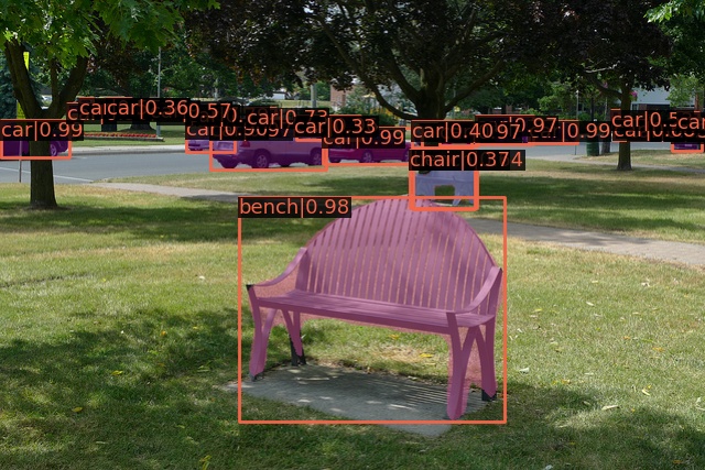
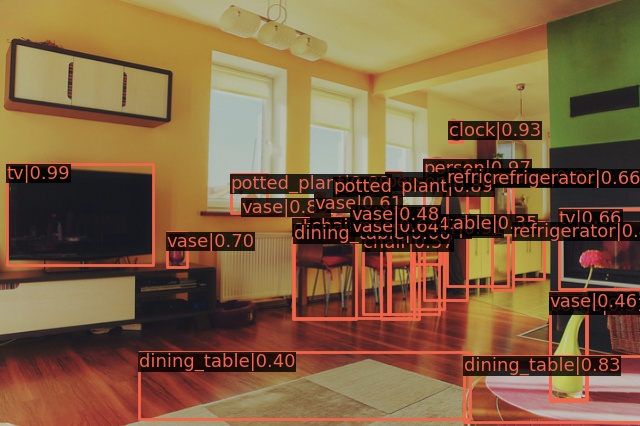
저장된 5000개의 이미지(COCO test, faster_rcnn) 중 하나를 가져와 보았다.

faster_rcnn_result.jpg

Test without Ground Truth Annotations

데이터셋 형식 변환

COCO 형식으로 변환하는 것을 기본으로 하는 것 같다.

다른 형식의 데이터셋은 다음 코드를 통해 COCO 형식으로 바꿀 수 있다.

python tools/dataset_converters/images2coco.py \
    ${IMG_PATH} \
    ${CLASSES} \
    ${OUT} \
    [--exclude-extensions]

파일 형식에 따라 다음 파일로 대체하면 된다.

변환을 완료했으면 다음 코드를 통해 GT annotation 없이 테스트를 해볼 수 있다.

# single-gpu testing
python tools/test.py \
    ${CONFIG_FILE} \
    ${CHECKPOINT_FILE} \
    --format-only \
    --options ${JSONFILE_PREFIX} \
    [--show]

1. Train predefined models on standard datasets

데이터셋 등은 위에서 설명한 대로 준비해 놓자.

학습하는 코드는 다음과 같다.

# single GPU
python tools/train.py \
    ${CONFIG_FILE} \
    [optional arguments]
# Multiple GPUs
bash ./tools/dist_train.sh \
    ${CONFIG_FILE} \
    ${GPU_NUM} \
    [optional arguments]

# 예시
python tools/train.py \
    configs/faster_rcnn/faster_rcnn_r50_fpn_2x_coco.py 
    --work-dir work_dir_tutorial_2

bash ./tools/dist_train.sh  
    configs/faster_rcnn/faster_rcnn_r50_fpn_2x_coco.py 
    2

log 파일과 checkpoint는 work_dir/ 또는 --work-dir로 지정한 디렉토리에 생성된다.

config 파일만 지정하면 알아서 학습이 진행된다. 실행 환경 정보, 모델, optimizer, 평가방법 등 config 정보 등이 출력되며 학습이 시작된다.
기본적으로 evaluation을 매 epoch마다 진행하는데, 이는 추가 옵션으로 바꿀 수 있다.

  • 1개의 Titan X로는 5일 7시간, 2개로는 3일 8시간 정도 소요된다고 나온다.

위에서 설명한 페이지 아래쪽에는 이외에도 여러 개의 job을 동시에 돌리는 법, Slurm으로 돌리는 방법 등이 공식 홈페이지에 있으니 쓸 생각이 있으면 참조하면 된다.


2: Train with customized datasets

다른 데이터셋을 가져와서 학습하는 방법을 설명하는데, 다음 단계를 따르면 된다.

  1. 사용할 데이터셋을 준비한다. annotation을 COCO format으로 변환하면 편하다.
  2. Config 파일을 수정한다.
  3. 준비한 데이터셋에서 학습과 추론을 진행한다.

여기서는 balloon dataset을 COCO format으로 변환한 다음 학습하는 방법을 설명한다.

Annotation 파일을 COCO format으로 변환

Balloon dataset의 annotation 파일은 대충 다음과 같이 생겼다.

{'base64_img_data': '',
 'file_attributes': {},
 'filename': '34020010494_e5cb88e1c4_k.jpg',
 'fileref': '',
 'regions': {'0': {'region_attributes': {},
   'shape_attributes': {'all_points_x': [1020,
     1000,
     994,
     ...
     1020],
    'all_points_y': [963,
     899,
     841,
     ...
     963],
    'name': 'polygon'}}},
 'size': 1115004}

COCO format은 다음과 같다.

 {
    "images": [image],
    "annotations": [annotation],
    "categories": [category]
}


image = {
    "id": int,
    "width": int,
    "height": int,
    "file_name": str,
}

annotation = {
    "id": int,
    "image_id": int,
    "category_id": int,
    "segmentation": RLE or [polygon],
    "area": float,
    "bbox": [x,y,width,height],
    "iscrowd": 0 or 1,
}

categories = [{
    "id": int,
    "name": str,
    "supercategory": str,
}]

그러니 Balloon dataset의 annotation 파일(json 파일)을 COCO format으로 변환하는 코드가 필요하다.

  • 참고: 공식 홈페이지 코드에는 어째 import mmcv가 빠져 있다.
import os.path as osp
import mmcv

def convert_balloon_to_coco(ann_file, out_file, image_prefix):
    data_infos = mmcv.load(ann_file)
    
    annotations = []
    images = []
    obj_count = 0
    for idx, v in enumerate(mmcv.track_iter_progress(data_infos.values())):
        filename = v['filename']
        img_path = osp.join(image_prefix, filename)
        height, width = mmcv.imread(img_path).shape[:2]
        
        images.append(dict(
            id=idx,
            file_name=filename,
            height=height,
            width=width))
        
        bboxes = []
        labels = []
        masks = []
        for _, obj in v['regions'].items():
            assert not obj['region_attributes']
            obj = obj['shape_attributes']
            px = obj['all_points_x']
            py = obj['all_points_y']
            poly = [(x + 0.5, y + 0.5) for x, y in zip(px, py)]
            poly = [p for x in poly for p in x]
            
            x_min, y_min, x_max, y_max = (
                min(px), min(py), max(px), max(py))
            
            
            data_anno = dict(
                image_id=idx,
                id=obj_count,
                category_id=0,
                bbox=[x_min, y_min, x_max - x_min, y_max - y_min],
                area=(x_max - x_min) * (y_max - y_min),
                segmentation=[poly],
                iscrowd=0)
            annotations.append(data_anno)
            obj_count += 1
    
    coco_format_json = dict(
        images=images,
        annotations=annotations,
        categories=[{'id':0, 'name': 'balloon'}])
    mmcv.dump(coco_format_json, out_file)


convert_balloon_to_coco('train/via_region_data.json',
                        'train/annotation_coco.json',
                        'train')

convert_balloon_to_coco('val/via_region_data.json',
                        'val/annotation_coco.json',
                        'val')

위의 코드를 다음과 같이 놓고 실행하면 변환이 완료된다.

balloon
├── convert_annotations.py
├── train
│   ├── *.jpg
│   ├── via_region_data.json
│   ├── annotation_coco.json
├── val
│   ├── *.jpg
│   ├── via_region_data.json
│   ├── annotation_coco.json

결과:

root@0d813b2889d8:/mmdetection/data/balloon# python convert_annotation.py 
[>>>>>>>>>>>>>>>>>>>>>>>>>>>>>>>>>>>>>>>>>>>>>>>>>>] 61/61, 49.4 task/s, elapsed: 1s, ETA:     0s
[>>>>>>>>>>>>>>>>>>>>>>>>>>>>>>>>>>>>>>>>>>>>>>>>>>] 13/13, 48.6 task/s, elapsed: 0s, ETA:     0s

Config 파일 준비

mmdetection/configs/balloon/ 디렉토리를 만들고 mask_rcnn_r50_caffe_fpn_mstrain-poly_1x_balloon.py 파일을 생성한다. Mask R-CNN with FPN 모델을 사용하기 때문에 이러한 이름을 가진다.

파일 내용은 다음과 같다.

# The new config inherits a base config to highlight the necessary modification
_base_ = '../mask_rcnn/mask_rcnn_r50_caffe_fpn_mstrain-poly_1x_coco.py'

# We also need to change the num_classes in head to match the dataset's annotation
model = dict(
    roi_head=dict(
        bbox_head=dict(num_classes=1),
        mask_head=dict(num_classes=1)))

# Modify dataset related settings
dataset_type = 'COCODataset'
classes = ('balloon',)
data = dict(
    train=dict(
        img_prefix='data/balloon/train/',
        classes=classes,
        ann_file='data/balloon/train/annotation_coco.json'),
    val=dict(
        img_prefix='data/balloon/val/',
        classes=classes,
        ann_file='data/balloon/val/annotation_coco.json'),
    test=dict(
        img_prefix='data/balloon/val/',
        classes=classes,
        ann_file='data/balloon/val/annotation_coco.json'))

# We can use the pre-trained Mask RCNN model to obtain higher performance
load_from = 'checkpoints/mask_rcnn_r50_caffe_fpn_mstrain-poly_3x_coco_bbox_mAP-0.408__segm_mAP-0.37_20200504_163245-42aa3d00.pth'

학습 및 추론하기

Checkpoint 파일을 받아서 checkpoints/ 안에 둔다.

현재 디렉토리 구조는 다음과 같다. 위치가 다르다면 경로를 수정해도 된다.

mmdetection
├── mmdet
├── tools
├── configs
│   ├── balloon
│   │   ├── mask_rcnn_r50_caffe_fpn_mstrain-poly_1x_balloon.py
│   ├── mask_rcnn
│   │   ├── mask_rcnn_r50_caffe_fpn_1x_coco.py
│   │   ├── mask_rcnn_r50_fpn_1x_coco.py'
│   │   ├── ...
├── checkpoints
│   ├── faster_rcnn_r50_fpn_1x_coco_20200130-047c8118.pth
│   ├── mask_rcnn_r50_caffe_fpn_mstrain-poly_3x_coco_bbox_mAP-0.408__segm_mAP-0.37_20200504_163245-42aa3d00.pth
├── data
│   ├── balloon
│   │   ├── convert_annotations.py
│   │   ├── train
│   │   │   ├── *.jpg
│   │   │   ├── annotation_coco.json
│   │   ├── val
│   │   │   ├── *.jpg
│   │   │   ├── annotation_coco.json

이제 학습을 진행하면 된다.

python tools/train.py configs/balloon/mask_rcnn_r50_caffe_fpn_mstrain-poly_1x_balloon.py

결과:

...
2021-09-03 06:37:20,209 - mmdet - INFO - Saving checkpoint at 12 epochs
2021-09-03 06:37:20,690 - mmdet - INFO - Exp name: mask_rcnn_r50_caffe_fpn_mstrain-poly_1x_balloon.py
2021-09-03 06:37:20,690 - mmdet - INFO - Epoch(val) [12][13]    bbox_mAP: 0.7080, 
bbox_mAP_50: 0.8280, bbox_mAP_75: 0.7820, bbox_mAP_s: 0.2020, bbox_mAP_m: 0.4750, 
bbox_mAP_l: 0.8110, bbox_mAP_copypaste: 0.708 0.828 0.782 0.202 0.475 0.811, 
segm_mAP: 0.7460, segm_mAP_50: 0.8190, segm_mAP_75: 0.7740, segm_mAP_s: 0.4040, 
segm_mAP_m: 0.4850, segm_mAP_l: 0.8350, segm_mAP_copypaste: 0.746 0.819 0.774 0.404 0.485 0.835

이제 work_dirs에는 다음과 같이 파일들이 생성되어 있다. 명령창에서 --work-dirs 옵션을 주었다면 해당 디렉토리로 들어가면 된다.

mmdetection
├── work_dirs
│   ├── mask_rcnn_r50_caffe_fpn_mstrain-poly_1x_balloon
│   │   ├── 20210903_061911.log  
│   │   ├── ...
│   │   ├── 20210903_062541.log  
│   │   ├── 20210903_063427.log.json  
│   │   ├── epoch_1.pth   
│   │   ├── epoch_2.pth  
│   │   ├── ...
│   │   ├── epoch_12.pth  
│   │   ├── latest.pth
│   │   ├── mask_rcnn_r50_caffe_fpn_mstrain-poly_1x_balloon.py

latest.pth 파일을 이용해서 테스트를 진행하려면 다음과 같이 입력한다.

python tools/test.py \
    configs/balloon/mask_rcnn_r50_caffe_fpn_mstrain-poly_1x_balloon.py \
    work_dirs/mask_rcnn_r50_caffe_fpn_mstrain-poly_1x_balloon/latest.pth \
    --eval bbox segm \
    --show-dir results/mask_rcnn_r50_caffe_fpn_mstrain-poly_1x_balloon
  • 참고: 공식 코드에는 어째서인지 디렉토리 이름을 ...balloon.py\latest.path로 적어 놨다… 대규모 프로젝트의 코드치고 자잘한 오류가 많다.

대략 다음과 같은 결과를 얻을 수 있다.

OrderedDict([
    ('bbox_mAP', 0.708), ('bbox_mAP_50', 0.828), ('bbox_mAP_75', 0.782),
    ('bbox_mAP_s', 0.202), ('bbox_mAP_m', 0.475), ('bbox_mAP_l', 0.811), 
    ('bbox_mAP_copypaste', '0.708 0.828 0.782 0.202 0.475 0.811'), ('segm_mAP', 0.746), 
    ('segm_mAP_50', 0.819), ('segm_mAP_75', 0.774), ('segm_mAP_s', 0.404), 
    ('segm_mAP_m', 0.485), ('segm_mAP_l', 0.835), 
    ('segm_mAP_copypaste', '0.746 0.819 0.774 0.404 0.485 0.835')
])

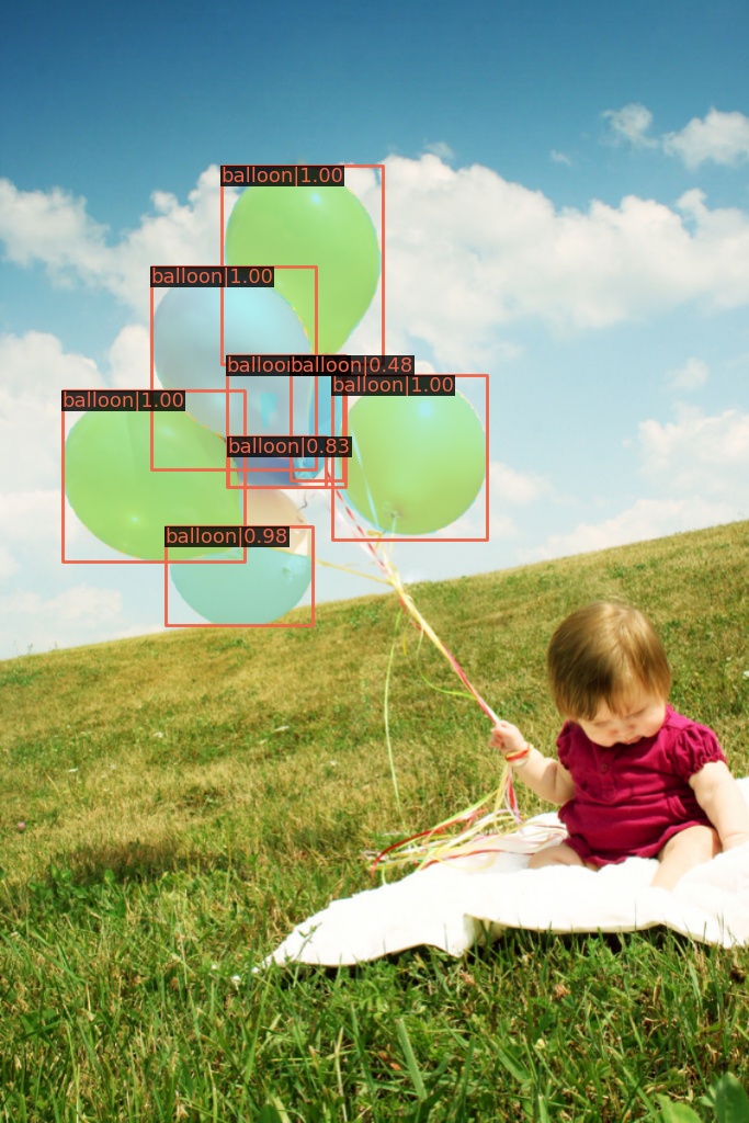
이제 mmdetection/results/mask_rcnn_r50_caffe_fpn_mstrain-poly_1x_balloon 디렉토리에 들어가보면 data/balloon/val 안에 있던 13개의 이미지에 대해 bbos를 친 결과를 확인할 수 있다.

balloon_result.jpg

3: Train with customized models and standard datasets

CityScapes와 같은 표준 데이터셋에 사용자 모델을 학습시키려면 다음 과정을 따른다.

  1. 표준 데이터셋을 준비한다.
  2. 사용자 모델을 준비한다.
  3. Config 파일을 생성한다.
  4. 표준 데이터셋에서 사용자 모델을 학습 및 추론한다.

CityScapes 데이터셋 준비

  • 참고: 이 부분은 미구현된 부분이 있어서 그대로는 동작하지 않는다.

먼저 다운로드를 해야 한다. 학교 이메일 등으로만 회원가입이 된다(gmail 불가).

홈페이지에서 다음을 받으면 된다.

  • leftImg8bit_trainvaltest.zip (11GB)
  • gtFine_trainvaltest.zip (241MB)

참고로 annotations은 각각의 데이터셋 안에 들어 있으니 따로 추가로 받아야 할 것은 없다.

CityScapes는 위에서 설명했던 것과 같이 데이터셋은 다음과 같은 구조로 둔다.

mmdetection
├── mmdet
├── tools
├── configs
├── data
│   ├── coco
│   │   ├── annotations
│   │   ├── train2017
│   │   ├── val2017
│   │   ├── test2017
│   ├── cityscapes
│   │   ├── annotations
│   │   ├── leftImg8bit
│   │   │   ├── train
│   │   │   ├── val
│   │   ├── gtFine
│   │   │   ├── train
│   │   │   ├── val
│   ├── VOCdevkit
│   │   ├── VOC2007
│   │   ├── VOC2012

CityScapes류 데이터셋은 COCO format으로 변환하는 과정이 필요하다.

pip install cityscapesscripts
python tools/dataset_converters/cityscapes.py ./data/cityscapes --nproc 8 --out-dir ./data/cityscapes/annotations

그러면 간단히 변환이 완료된다.

Converting train into instancesonly_filtered_gtFine_train.json
Loaded 2975 images from ./data/cityscapes/leftImg8bit/train
Loading annotation images
[>>>>>>>>>>>>>>>>>>>>>>>>>>>>>>>>>>>>>>>>>>>>>>>>>>] 2975/2975, 30.1 task/s, elapsed: 99s, ETA:     0s
It took 100.40516328811646s to convert Cityscapes annotation

사용자 모델 준비

여기서는 Cascade Mask R-CNN R50 모델을 기반으로 하는 모델을 사용자 모델로 쓴다. 이 모델을 그대로 쓰는 것은 아니고 FPNAugFPN으로, training time auto augmentation으로 RotateTranslate를 추가하는 변형을 가한다.

새 파일 mmdet/models/necks/augfpn.py을 만든다.

from ..builder import NECKS

@NECKS.register_module()
class AugFPN(nn.Module):

    def __init__(self,
                in_channels,
                out_channels,
                num_outs,
                start_level=0,
                end_level=-1,
                add_extra_convs=False):
        pass

    def forward(self, inputs):
        # implementation is ignored
        pass

그리고 mmdet/models/necks/__init__.py 파일에 from .augfpn import AugFPN 코드를 추가하거나,

config 파일에 다음을 추가하면 된다.

custom_imports = dict(
    imports=['mmdet.models.necks.augfpn.py'],
    allow_failed_imports=False)

__init__.py 파일은 다음과 같이 생겼다.

사용자 모델을 설계하는 방법이나 학습 세팅에 대한 더 자세한 정보는 다음 링크를 참고하자.

Config 파일 준비

이제 configs/cityscapes/cascade_mask_rcnn_r50_augfpn_autoaug_10e_cityscapes.py 파일을 생성하자.

config 파일의 코드는 여기를 참조하자.

학습 및 추론

python tools/train.py configs/cityscapes/cascade_mask_rcnn_r50_augfpn_autoaug_10e_cityscapes.py
python tools/test.py configs/cityscapes/cascade_mask_rcnn_r50_augfpn_autoaug_10e_cityscapes.py work_dirs/cascade_mask_rcnn_r50_augfpn_autoaug_10e_cityscapes.py/latest.pth --eval bbox segm

Tutorials에 대한 설명은 다음 글에서..

Comment  Read more