EM (Expected Maximization) 알고리즘 설명
28 Jul 2020 | Machine_Learning이번 글에서는 통계학을 비롯하여 여러 분야에서 중요하게 사용되는 Expected Maximization 알고리즘에 대해 설명하도록 할 것이다. 본 글은 Bishop의 Pattern Recognition And Machine Learning Chapter9 부분을 번역하여 정리한 것이다. 더욱 상세한 내용을 원한다면 직접 책을 참고하면 좋을 것이다.
EM 알고리즘은 잠재 변수를 가진 모델에서 MLE를 찾는 일반적인 방법이다. Stochastic Gradient Descent와 같은 함수 최적화 방식으로 MLE를 찾을 수 있지만 쉽게 이해하고 구현할 수 있다는 장점을 바탕으로 여전히 널리 사용되고 있는 알고리즘이다.
1. Mixture Models
1.1. Mixture of Gaussians
Gaussian Mixture Model을 이산적인 잠재 변수를 갖는 모델로서 생각해보자. Gaussian Mixture 분포는 아래와 같이 정규분포의 선형 결합으로 표현될 수 있다.
| [p(\mathbf{x}) = \Sigma_{k=1}^K \pi_k \mathcal{N} (\mathbf{x} | \mu_k, \Sigma_k)] |
이 때 $\pi_k$ 는 k라는 cluster에 속할 확률을, $K$ 는 Cluster의 개수를 의미한다.
위와 같이 표현이 가능한 이유에 대해 알아보자. 1-of-K representation(하나의 원소만 1이고, 나머지는 0인)을 갖고 $K$ 차원을 가진 이산 확률 변수 $\mathbf{z}$ 가 있다고 하자.
우리는 이제 결합확률 분포 $p(\mathbf{x}, \mathbf{z})$ 를 아래 두 분포의 관점에서 정의하고자 한다. (베이지안 관점에서 생각해보면 된다.)
| [p(\mathbf{z}), p(\mathbf{x} | \mathbf{z})] |
$\mathbf{z}$ 에 대한 Marginal 분포는 아래와 같이 mixing 계수 $\pi_k$ 의 관점에서 구체화될 수 있다.
[p(z_k = 1) = \pi_k]
$\mathbf{z}$ 가 1-of-K representation을 갖고 있기 때문에 우리는 다음과 같이 $p(\mathbf{z})$ 를 정의할 수 있다.
[p(\mathbf{z}) = \prod_{k=1}^K \pi_k^{z_k}]
유사하게, 특정 $\mathbf{z}$ 값이 주어졌을 때 $\mathbf{x}$ 의 조건부 분포는 아래와 같이 정규분포이다.
| [p(\mathbf{x} | z_k = 1) = \mathcal{N} (\mathbf{x} | \mu_k, \Sigma_k)] |
이 사실을 이용하여 다음의 결과를 얻을 수 있다.
| [p(\mathbf{x} | \mathbf{z}) = \prod_{k=1}^K \mathcal{N} (\mathbf{x} | \mu_k, \Sigma_k)^{z_k}] |
최종적으로 이번 Chapter 서두에서 보았던 $p(\mathbf{x})$ 를 얻을 수 있다.
| [p(\mathbf{x}) = \Sigma_z p(\mathbf{z}) p(\mathbf{x} | \mathbf{z}) =\Sigma_{k=1}^K \pi_k \mathcal{N} (\mathbf{x} | \mu_k, \Sigma_k)] |
각 $x_i$ 에 대해 이에 상응하는 $z_i$ 가 존재한다는 사실을 알 수 있다. 이제 명시적인 잠재 변수를 포함하는 Gaussian Mixture 공식을 얻긴 하였는데, 사실 우리는 $p(\mathbf{x}, \mathbf{z})$ 를 얻고 싶다. 이는 EM 알고리즘을 통해 수행될 수 있다.
Posterior 또한 매우 중요하다. $\mathbf{x}$ 가 주어졌을 때 $z_k = 1$ 일 조건부 확률을 $\gamma(z_k)$ 라고 하자. 베이즈 정리에 의해 다음 식을 도출할 수 있다.
| [\gamma(z_k) = p(z_k = 1 | \mathbf{x}) = \frac {p(z_k = 1) p(\mathbf{x} | z_k = 1)} {\Sigma_{j=1}^K p(z_j = 1) p(\mathbf{x} | z_j = 1)}] |
| [= \frac {\pi_k \mathcal{N} (\mathbf{x} | \mu_k, \Sigma_k ) } {\Sigma_{j=1}^K \pi_j \mathcal{N} (\mathbf{x} | \mu_j, \Sigma_j)}] |
이제 이 $\gamma(z_k)$ 는 관측값 x를 설명하는 데에 있어 component k의 Responsibility로 파악할 수 있다.
1.2. Maximum Likelihood
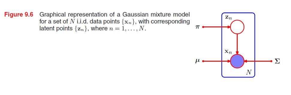
우리가 $\mathbf{x}_1, …, \mathbf{x}_N$ 의 관측값을 가진 데이터셋을 갖고 있다고 하자. 그리고 우리는 GMM을 이용하여 이 $(N, D)$ 형상의 데이터 $X$를 모델링하고 싶다. 이 때 n번째 행은 $\mathbf{x}_n^T$ 라고 표현될 수 있을 것이다.
유사하게도 이에 상응하는 잠재 변수들은 $(N, K)$ 형상의 $Z$ 행렬로 표현될 수 있고, 이 때 행은 $\mathbf{z}_n^T$ 라고 표현할 수 있을 것이다. 모든 데이터가 분포로부터 독립적으로 추출되었다면, 우리는 GMM을 다음과 같은 그래프 모델로 표현할 수 있다.
이 때 Log Likelihood 함수는 아래와 같이 표현될 수 있다.
| [log p(\mathbf{X} | \pi, \mu, \Sigma) = \Sigma_{n=1}^N log [\Sigma_{k=1}^K \pi_k \mathcal{N} ( \mathbf{x}_n | \mu_k, \Sigma_k ) ]] |
이제 MLE를 통해서 이 함수를 최대화 해야 한다. 그런데 그게 그렇게 녹록치만은 않다. 2가지 이슈가 있다.
1) 특이점 문제: Problem of Singularities
2) 혼합의 식별 문제: Indentifiability of Mixtures
먼저 특이점 문제에 대해 살펴볼 것인데, 공분산 행렬이 $\Sigma_k = \sigma^2_k I$ 인 간단한 Gaussiam Mixture에 대해 생각해보자.
이 때 j번째 분포만을 고려한다면 이 분포의 평균은 당연히 $\mu_j$ 일 것인데, 그런데 만약 이 j번째 분포에 오직 1개의 Sample만이 존재한다고 생각해보자.
그렇다면 $\mu_j = \mathbf{x}_n$ 가 될 것이고 Likelihood 함수는 다음과 같이 표현될 수 있다.
| [\mathcal{N} (\mathbf{x}_n | \mathbf{x}_n, \sigma_j^2 \mathbf{I}) = \frac{1}{(2\pi)^{\frac{1}{2}}\sigma_j}] |
만약 이 때 $\sigma_j \to 0$ 이라면, 이 항이 무한을 향해 나아갈 것이고 또한 Log Likelihood 또한 무한이 될 것이다. (Likelihood 함수는 각각의 분포의 곱으로 표현된다.)
따라서 이러한 형태의 Likelihood 함수는 well-posed된 문제라고 할 수 없다. 왜냐하면 이러한 Singularities는 Gaussian Component들 중 하나라도 특정 데이터 포인트에 쏠리기만 해도 이러한 현상은 언제나 발생하기 때문이다.
단 하나의 Gaussian에서는 이러한 문제가 거의 발생하지 않지만, Gaussian Mixture에서는 우연히 하나의 데이터 포인트가 하나의 분포를 이루는 경우가 종종 존재하기 때문에 문제가 되는 것이다.
이러한 Singularity는 Maximum Likelihood 방법론에서 발생할 수 있는 심각한 과적합 문제에 대한 또다른 예시를 제공해주는 셈이다. 우리가 만약 Bayesian Approach를 도입한다면 이러한 문제를 겪지 않을 수 있다. 적절한 휴리스틱을 도입함으로써 이러한 문제를 해결할 수 있는데, 예를 들어 Gaussian Component가 평균이 특정 데이터 포인트에 collapse할 경우 그 component의 평균을 랜덤하게 선택된 값으로 설정하고, 공분산 역시 어떤 큰 값으로 설정한 후 최적화를 다시 진행할 수 있을 것이다.
이제 두 번째 문제인 식별 문제에 대해 알아보자. K개의 파라미터를 K개의 Component에 할당하는 방법은 K!개이기 때문에, K-component Mixture에는 MLE 결과를 동일하게 만드는 K!개의 Solution이 발생하게 된다.
따라서 임의의 한 Sample에 대해 똑같은 분포를 만들어 낼 수 있는 K!-1 개의 데이터 포인트가 존재하게 된다. 이러한 문제를 식별 문제, Identifiability라고 부르며 모델에 의해 밝혀진 파라미터를 해석하는 데에 있어서 굉장히 중요한 이슈이다.
1.3. EM for Gaussian Mixtures
다음 Chapter에서는 EM 알고리즘이 변분 추론의 한 방법임을 밝히면서 좀 더 일반화된 설명을 진행하겠지만, 일단 이번 Chapter에서는 GMM의 맥락에서 설명하도록 하겠다.
GMM을 EM 알고리즘으로 풀어내기 위해서는 Log Likelihood를 최대화하는 파라미터들인 $\mu, \Sigma, \pi$ 를 찾아내야 한다. 지금부터 차근차근 단계를 밟아나가 보도록 하겠다.
| [log p(\mathbf{X} | \pi, \mu, \Sigma) = \Sigma_{n=1}^N log (\Sigma_{k=1}^K \pi_k \mathcal{N} ( \mathbf{x}_n | \mu_k, \Sigma_k ))] |
Gaussian Component의 평균 $\mu_k$ 에 대한 위 식의 미분 값을 0이라고 설정하면 우리는 다음 식을 얻을 수 있다.
| [0 = - \Sigma_{n=1}^N \frac{\pi_k \mathcal{N} ( \mathbf{x}_n | \mu_k, \Sigma_k )}{\Sigma_{j} \pi_j \mathcal{N} ( \mathbf{x}_n | \mu_j, \Sigma_j )} \Sigma_k (\mathbf{x}_n - \mu_k)] |
이 때 중간의 분수 식은 $\gamma(z_{nk})$ 임을 기억하자. $\Sigma_k^{-1}$ 를 곱하고 정리하면 다음을 얻을 수 있다. 이 식을 A 식이라고 하자.
[\mu_k = \frac{1}{N_k} \Sigma_{n=1}^N \gamma(z_{nk}) \mathbf{x}_n]
[N_k = \Sigma_{n=1}^N \gamma(z_{nk})]
이 때 $N_k$ 는 Cluster k에 배정된 데이터 포인트의 효과적인 수로 해석할 수 있다. k번째 Gaussian Component의 평균 $\mu_k$ 는 데이터셋에 있는 모든 데이터 포인트의 가중 평균을 취함으로써 얻을 수 있다.
이 때 데이터 포인트 $\mathbf{x}_n$ 의 가중 Factor는,
Component k가 $\mathbf{x}_n$ 을 생성하는 데 Responsible할 사후 확률을 의미하며 그 확률은 아래와 같다.
[\gamma(z_{nk})]
이번에는 $\Sigma_k$ 에 대한 Log Likelihood의 미분 값을 0이라고 설정하고 위와 같은 유사한 과정을 거치면 single Gaussian에 대한 공분산 행렬의 Maximum Likelihood Solution을 아래와 같이 얻을 수 있다. 이 식을 B 식이라고 하자.
[\Sigma_k = \frac{1}{N_k} \Sigma_{n=1}^N \gamma(z_{nk}) (\mathbf{x}_n - \mu_k) (\mathbf{x}_n - \mu_k)^T]
위 식은 데이터셋에 적합한 single Gaussian의 결과와 같은 형상을 취하지만, 각 데이터 포인트는 상응하는 사후 확률에 의해 가중되어 있고, 각 Component의 데이터 포인트의 효과적인 수로 나눠지고 있다.
이제 마지막으로 이 Log Likelihood를 mixing 계수 $\pi_k$ 에 대해 최대화해보자. 이 때 mixing 계수들의 총합은 1이라는 조건이 만족되어야 하는데, 이는 Lagrange Multiplier를 사용하는 것으로 해결할 수 있다.
| [log p(\mathbf{x} | \pi, \mu, \Sigma) + \lambda (\Sigma_{k=1}^K \pi_k - 1 )] |
그래서 위 식을 최대화하면,
| [0 = \Sigma_{n=1}^N \frac{\mathcal{N} ( \mathbf{x}_n | \mu_k, \Sigma_k )}{\Sigma_{j} \pi_j \mathcal{N} ( \mathbf{x}_n | \mu_j, \Sigma_j )} + \lambda] |
이 때 $\pi_k$ 를 양변에 곱해주면,
| [0 = \Sigma_{n=1}^N \frac{\pi_k \mathcal{N} ( \mathbf{x}_n | \mu_k, \Sigma_k )}{\Sigma_{j} \pi_j \mathcal{N} ( \mathbf{x}_n | \mu_j, \Sigma_j )} + \lambda] |
[\to 0 = \Sigma_{n=1}^N \gamma(r_{nk}) + \lambda]
[\to 0 = N_k + \lambda]
$\lambda = N_k$ 임을 알았다. $\lambda$ 대신 $N_k$ 를 이용하여 식을 다시 정리하면, 아래와 같은 결과를 얻을 수 있다. 이 식은 C 식이라고 하자.
[\pi_k = \frac{N_k}{N}]
해석해보면, k번째 Component의 mixing 계수는 그 Component가 데이터 포인트들을 설명하는 평균 Responsiblity를 의미한다고 볼 수 있다.
이렇게 얻은 $\mu_k, \Sigma_k, \pi_k$ 는 Closed-form의 해를 갖지 못하느데, 왜냐하면 이 파라미터들은 아래 식에서처럼 $\gamma(z_k)$ 에 영향을 받기 때문이다.
| [\gamma(z_k) = p(z_k = 1 | \mathbf{x}) = \frac {\pi_k \mathcal{N} (\mathbf{x} | \mu_k, \Sigma_k ) } {\Sigma_{j=1}^K \pi_j \mathcal{N} (\mathbf{x} | \mu_j, \Sigma_j)}] |
따라서 MLE를 얻기 위해서는 Iterative(반복적인) 방법이 제안된다. 일단 처음에는 이 파라미터들에 대한 초깃값을 설정하고, E step과 M step이라 부르는 2가지 단계를 통해 업데이트를 교대로 수행하면 된다.
먼저 E step에서는 위 $\gamma(z_k)$ 에 대한 식을 통해 파라미터의 현재의 값으로 사후 확률을 평가한다. 그리고 이 확률은 M step에서 파라미터들을 A, B, C 식으로 재추정하는데에 사용된다.
정리해보자.
EM for Gaussian Mixtures
1) 평균, 공분산, mixing 계수를 초기화하고 Log Likelihood의 초깃값을 평가한다.
2) E step: 현재의 파라미터 값에 기반하여 Responsibility를 구한다.
| [\gamma(z_k) = \frac {\pi_k \mathcal{N} (\mathbf{x} | \mu_k, \Sigma_k ) } {\Sigma_{j=1}^K \pi_j \mathcal{N} (\mathbf{x} | \mu_j, \Sigma_j)}] |
3) M step: 위에서 구한 Responsibility와 A, B, C 식을 바탕으로 새로운 파라미터값을 재추정한다.
[\mu_k = \frac{1}{N_k} \Sigma_{n=1}^N \gamma(z_{nk}) \mathbf{x}_n]
[\Sigma_k = \frac{1}{N_k} \Sigma_{n=1}^N \gamma(z_{nk}) (\mathbf{x}_n - \mu_k) (\mathbf{x}_n - \mu_k)^T]
[\pi_k = \frac{N_k}{N}]
4) Log Likelihood를 평가한다.
| [log p(\mathbf{X} | \pi, \mu, \Sigma) = \Sigma_{n=1}^N log [\Sigma_{k=1}^K \pi_k \mathcal{N} ( \mathbf{x}_n | \mu_k, \Sigma_k ) ]] |
그리고 파라미터나 Log Likelihood가 수렴하는지 확인한다. 만약 수렴하지 않는다면, 계속해서 2단계로 돌아가서 반복한다.
2. An Alternative View of EM
이번 Chapter에서는 EM 알고리즘에서 잠재 변수가 갖는 핵심적인 역할에 대해 살펴볼 것이다.
다시 설명하지만, EM 알고리즘의 목표는 잠재 변수를 갖는 모델의 Maximum Likelihood를 찾는 것이다. 파라미터가 주어졌을 때 Log Likelihood는 아래와 같다.
| [log p(\mathbf{X} | \theta) = log { \Sigma_{\mathbf{Z}} p (\mathbf{X}, \mathbf{Z} | \theta) }] |
물론 연속적인 잠재 변수가 존재하면 위 식에 적분 기호를 적용하면 된다.
중요한 점은, 잠재 변수에 대한 $\Sigma$ 가 Log 안쪽에 있다는 것이다. 이 부분은 Logarithm이 결합 분포에 직접적으로 영향을 미치는 것을 막아 Maximum Likelihood Solution을 찾는 데 있어서 어려움을 가져다 준다.
잠시 Complete 과 Incomplete의 개념을 알아보자. $\mathbf{Z}, \mathbf{X}$ 를 모두 알고 있다면, 이를 Complete 데이터라고 부른다. 만약 잠재 변수에 대해서는 알지 못하고 $\mathbf{X}$ 에 대해서만 안다면, 이는 Incomplete 데이터이다.
| [log p(\mathbf{X, Z} | \theta)] |
이 때 Complete 데이터의 경우 Likelihood 함수는 단지 위 식과 같이 표현되기 때문에 계산이 어렵지 않다.
그러나 실제로 $\mathbf{Z}$ 를 아는 경우는 매우 드물다. 우리가 잠재 변수에 대해 아는 것은 오직 Posterior일 뿐이다. 우리가 Complete-data Log Likelihood를 쓸 수 없기 때문에, 잠재 변수의 사후 분포 하의 이것의 기댓값을 사용하는 것을 생각해 보아야 하는데, 이는 사실 E step에 해당하는 부분이다.
이어지는 M step에서는 이 기댓값을 최대화 한다. 만약 파라미터에 대한 현재의 추정값을 $\theta^{old}$ 라고 한다면, E, M step 이후의 파라미터는 $\theta^{new}$ 로 수정되어 표현할 수 있겠다.
E step 에서는 $\theta^{old}$를 사용하여 아래와 같은 잠재 변수에 대한 Posterior를 찾게 된다.
| [p(\mathbf{Z | X, \theta^{old}})] |
그리고 이 Posterior를 사용하여 어떤 일반적인 파라미터 값인 $\theta$ 를 찾기 위해 Complete-data Log Likelihood의 기댓값을 계산하게 된다. 이 기댓값은 $\mathcal{Q} (\theta, \theta^{old})$ 라고 표현하며 아래와 같은 형상을 취한다.
| [\mathcal{Q} (\theta, \theta^{old}) = \Sigma_{\mathbf{Z}} p(\mathbf{Z | X, \theta^{old}}) log p(\mathbf{X, Z | \theta})] |
그리고 M step에서는 위 식을 최대화하는 $\theta$ 를 찾아 $\theta^{new}$ 로 설정한다.
[\theta^{new} = \underset{\theta}{argmax} \mathcal{Q} (\theta, \theta^{old})]
$\mathcal{Q} (\theta, \theta^{old})$ 에서 Logarithm은 결합 분포에 직접적으로 영향을 미치기 때문에, M step 에서의 최적화는 tractable하다.
요약하자면 아래와 같다.
The General EM Algorithm
1) $\theta^{old}$ 에 대한 초깃값을 설정한다.
2) E step: 아래 사후 확률을 계산한다.
| [p(\mathbf{Z | X, \theta^{old}})] |
3) M step: $\theta^{new}$ 를 찾고 평가한다.
[\theta^{new} = \underset{\theta}{argmax} \mathcal{Q} (\theta, \theta^{old})]
| [\mathcal{Q} (\theta, \theta^{old}) = \Sigma_{\mathbf{Z}} p(\mathbf{Z | X, \theta^{old}}) log p(\mathbf{X, Z | \theta})] |
4) 파라미터 또는 Log Likelihood가 수렴하는지 확인하고, 그렇지 않다면 $\theta^{old} \leftarrow \theta^{new}$ 로 업데이트를 진행한 후 2단계 부터 다시 진행한다.
파라미터에 대해 Prior $p(\theta)$ 가 정의된 모델에 대해 MAP Solution을 찾는 데에도 EM 알고리즘을 쓰일 수 있다. 이 때 E step은 위와 동일하며 M step의 경우 아래와 같이 약간의 수정이 가미된다.
[\mathcal{Q} (\theta, \theta^{old}) + logp(\theta)]
Prior가 절절히 선택된다면 MAP Solution을 찾는 방식으로 Singularities를 제거할 수 있다.
지금까지 잠재 변수에 대해 대응하는 방식으로써 EM 알고리즘을 설명하였는데, 사실 이 알고리즘은 결측값이 존재할 때 역시 적용될 수 있는 알고리즘이다. 이 부분에 대해서는 다른 참고 자료를 확인하길 바란다.
이번 Chapter의 내용을 바탕으로 GMM을 다시 한 번 설명한 부분은 Reference의 책의 442페이지를 참조하길 바란다.
3. The EM algorithm in General
이 Chapter의 주된 내용은 EM 알고리즘을 변분 추론의 관점에서 설명하는 것이다. 변분 추론에 대해서 알고 싶다면 이 글을 참조하라.
지금까지 계속 보았듯이 우리의 목적은 아래 Likelihood를 최대화하는 것이다.
| [p(\mathbf{X} | \theta) = \Sigma_\mathbf{Z} p(\mathbf{X, Z | \theta})] |
잠재 변수에 대한 분포 $q(\mathbf{Z})$ 를 설정하자. 어떻게든 이 분포에 대해 알 수 있다면 아래와 같은 식은 성립한다.
| [log p(\mathbf{X} | \theta) = \mathcal{L}(q, \theta) + KL(q | p)] |
| [\mathcal{L}(q, \theta) = \Sigma_Z q(\mathbf{Z}) log { \frac{p(\mathbf{X, Z | \theta})}{q(\mathbf{Z})} }] |
| [KL(q | p) = - \Sigma_\mathbf{Z} q(\mathbf{Z}) log { \frac{p(\mathbf{Z | X, \theta})}{q(\mathbf{Z})} }] |
위 식은 변분 추론에 대한 사전 지식이 있다면 자주 보았던 식일 것이다. 아래와 같은 확률의 곱셈 법칙을 이용하면,
| [log p(\mathbf{X, Z | \theta}) = log p(\mathbf{Z | X, \theta}) + log p(\mathbf{X | \theta})] |
위에서 기술한 ELBO식을 다시 정리할 수 있을 것이다.
EM 알고리즘은 2단계로 MLE를 찾는 알고리즘이다. 위에서 본 분해 식을 활용하여 Log Likelihood를 최대화해보자.
현재의 파라미터를 $\theta^{old}$ 라고 한다면, E step에서는 이를 고정한 채, ELBO $\mathcal{L} (q, \theta)$ 를 $q(\mathbf{Z})$ 에 대해 최대화할 것이다. 이 최대화 해는 쉽게 찾을 수 있다. 그 이유에 대해 설명하겠다.
일단 앞서 확인한 확률의 곱셈법칙으로 인해 $\theta^{old}$ 가 주어졌을 때 아래 식은 $\mathbf{Z}$ 에 의존하지 않는다는 것을 알 수 있다.
| [log p(\mathbf{X, Z | \theta}) = log p(\mathbf{Z | X, \theta}) + log p(\mathbf{X | \theta})] |
그렇다면 ELBO가 최대화된다는 뜻은 결국 KL-divergence가 최소화된다는 뜻이다. 이 경우는 곧 KL-divergence 식에 존재하는 두 분포가 유사해질 때 발생한다는 것을 알 수 있다. (아래 참조)
| [q(\mathbf{Z}) \approx p(\mathbf{Z | X, \theta^{old}})] |
이제 M step 에서는 $q(\mathbf{Z})$ 를 위 식과 같이 고정하고 ELBO를 최대화하여 $\theta^{new}$ 를 얻는다. 이는 결국 Log Likelihood를 증가시키는 길이 될 것이다.
조금 더 상세히 알아보자. ELBO는 아래와 같은 식인 것을 확인했다.
| [\mathcal{L}(q, \theta) = \Sigma_Z q(\mathbf{Z}) log { \frac{p(\mathbf{X, Z | \theta})}{q(\mathbf{Z})} }] |
자 이제 $q(\mathbf{Z})$ 를 고정해보자.
| [\mathcal{L}(q, \theta) = \Sigma_Z p(\mathbf{Z | X, \theta^{old}}) log p(\mathbf{X, Z | \theta}) - \Sigma_Z p(\mathbf{Z | X, \theta^{old}}) log p(\mathbf{Z | X, \theta^{old}})] |
[= \mathcal{Q} (\theta, \theta^{old}) + Const]
위 상수는 사실 그냥 q 분포에 대한 Negative Entropy이다. 결국 M step 에서 최대화하고 있는 것은 이전 Chapter에서 설명하였던 것처럼, Complete-Data Log Likelihood인 것이다. 물론 만약 아래와 같은 결합 분포가 Exponential Family에 속한다면 Log가 Exponential을 cancel하고 계산은 훨씬 간단해질 것이다.
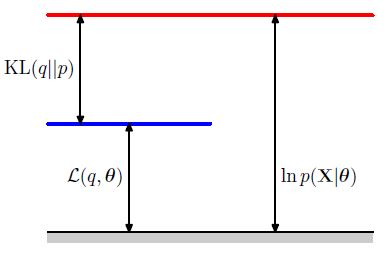
M step을 그림으로 나타내면 아래와 같다.
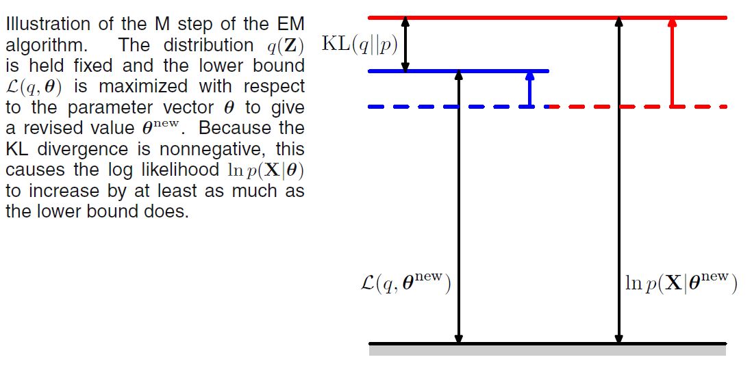
다음 그림은 EM 알고리즘의 전반적인 과정을 그림으로 표현한 것이다. 이와 같이 EM 알고리즘은 파라미터의 공간으로 해석할 수 있다. 이러한 측면 덕분에 EM 알고리즘은 Bayesian Optimization에서 Acqusiition Function으로 널리 사용되고 있다.
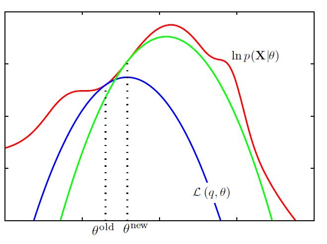
빨간 선이 우리가 최대화하고 싶은 Complete-Data Log Likelihood이다. 파란 선은 초깃값으로 설정한 ELBO이다. 지속적으로 EM을 수행하면 초록 선과 같은 결과를 얻을 수 있다.
References
Bishop, Pattern Recognition And Machine Learning, Chapter9